checkpointing: brms
chkpt_brms.RmdThe following examples walk through using chkptstanr
with the popular R package brms.
The basic idea is to (1) generate the Stan
code with brms, (2) fit the model with cmdstanr (with
the desired number of checkpoints), and then (3) return a
brmsfit object. This is all done internally, so the
workflow is very similar to using brms.
Example 1: No Stopping
Storage
The initial overhead is to create a folder that will store the checkpoints, i.e.,
path <- create_folder(folder_name = "chkpt_folder_m1")which contains several additional folders (details can be found in the documentation).
brmsformula
In this example, we create a brmsformula object using
bf(). Note that for this model, we could also use formula
argument (e.g., formula = y ~ x), but in our experiences
bf() is more general.
Model Fitting
The next step is to use chkpt_brms():
fit_m1 <- chkpt_brms(
  formula = bf_m1,
  data = epilepsy,
  path  = path,
  iter_warmup = 1000,
  iter_sampling = 1000,
  iter_per_chkpt = 250,
)
When running the above, a custom progress bar is printed that includes information about the checkpoints.
#> Compiling Stan program...
#> Initial Warmup (Typical Set)
#> Chkpt: 1 / 8; Iteration: 250 / 2000 (warmup)
#> Chkpt: 2 / 8; Iteration: 500 / 2000 (warmup)
#> Chkpt: 3 / 8; Iteration: 750 / 2000 (warmup)
#> Chkpt: 4 / 8; Iteration: 1000 / 2000 (warmup)
#> Chkpt: 5 / 8; Iteration: 1250 / 2000 (sample)
#> Chkpt: 6 / 8; Iteration: 1500 / 2000 (sample)
#> Chkpt: 7 / 8; Iteration: 1750 / 2000 (sample)
#> Chkpt: 8 / 8; Iteration: 2000 / 2000 (sample)
#> Checkpointing complete
In this case, checkpointing is complete.
Summary
fit_m1 is a brmsfit object which means that
all of the functionality of brms can still be used.
Here is the summary output:
fit_m1

#>  Family: poisson
#>   Links: mu = log
#> Formula: count ~ zAge + zBase + (1 | patient)
#>    Data: data (Number of observations: 236)
#>   Draws: 2 chains, each with iter = 1000; warmup = 0; thin = 1;
#>          total post-warmup draws = 2000
#>
#> Group-Level Effects:
#> ~patient (Number of levels: 59)
#>               Estimate Est.Error l-95% CI u-95% CI Rhat Bulk_ESS Tail_ESS
#> sd(Intercept)     0.58      0.07     0.46     0.73 1.00      349      682

#> Population-Level Effects:
#>           Estimate Est.Error l-95% CI u-95% CI Rhat Bulk_ESS Tail_ESS
#> Intercept     1.63      0.08     1.46     1.78 1.01      406      898
#> zAge          0.11      0.09    -0.06     0.27 1.00      463      796
#> zBase         0.73      0.08     0.58     0.89 1.00      613      814
#>
#> Draws were sampled using sample(hmc). For each parameter, Bulk_ESS
#> and Tail_ESS are effective sample size measures, and Rhat is the potential
#> scale reduction factor on split chains (at convergence, Rhat = 1).
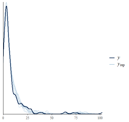
Posterior Predictive Check
Of course, due to being a brmsfit object, it is seamless
perform a posterior predictive check.
pp_check(fit_m1)
Example 2: Start, Stop, Start, etc.
The previous example could just as well be fitted directly with brms. This is because the MCMC sampler was not stopped during model fitting.
In the following example, we illustrate the usefulness of chkptstanr, i.e., the ability to stop the MCMC sampler at will, and then pick right back up where the MCMC sampler left off.
Storage
The initial overhead is to create a folder that will store the checkpoints, i.e.,
path <- create_folder(folder_name = "chkpt_folder_m2")Model Fitting
This model is mostly the same as above. The one difference is that it does not include varying (“random”) intercepts.
Start and Stop: Two Checkpoints
To illustrate checkpointing, the following was stopped after 2 checkpoints.
fit_m2 <- chkpt_brms(
  bf(formula = count ~ zAge + zBase,
            family = poisson()),
  data = epilepsy,
  path  = path,
  iter_warmup = 1000,
  iter_sampling = 1000,
  iter_per_chkpt = 250,
)

#> Compiling Stan program...
#> Initial Warmup (Typical Set)
#> Chkpt: 1 / 8; Iteration: 250 / 2000 (warmup)
#> Chkpt: 2 / 8; Iteration: 500 / 2000 (warmup)
Note this was stopped by clicking on the red button aptly titled stop (in the console).
This is but one use case, for example, needing to do something else but not wanting to loose the progress (including the compiled model). Another use case is scheduling, such that the model samples during certain times until completion.
Start and Stop: Two More Checkpoints
Now pick up at the next checkpoint. This is accomplished by simply running the same code.
fit_m2 <- chkpt_brms(
  formula = bf(formula = count ~ zAge + zBase,
               family = poisson()),
  data = epilepsy,
  path  = path,
  iter_warmup = 1000,
  iter_sampling = 1000,
  iter_per_chkpt = 250,
)

#> Sampling next checkpoint
#> Chkpt: 3 / 8; Iteration: 750 / 2000 (warmup)
#> Chkpt: 4 / 8; Iteration: 1000 / 2000 (warmup)
Notice it picks up at right where it left off (stopped after 2 checkpoints)
Start: Finish Checkpointing
Now let us finish the remaining 4 checkpoints.
fit_m2 <- chkpt_brms(
  formula = bf(formula = count ~ zAge + zBase,
               family = poisson()),
  data = epilepsy,
  path  = path,
  iter_warmup = 1000,
  iter_sampling = 1000,
  iter_per_chkpt = 250,
)

#> Sampling next checkpoint
#> Chkpt: 5 / 8; Iteration: 1250 / 2000 (sample)
#> Chkpt: 6 / 8; Iteration: 1500 / 2000 (sample)
#> Chkpt: 7 / 8; Iteration: 1750 / 2000 (sample)
#> Chkpt: 8 / 8; Iteration: 2000 / 2000 (sample)
#> Checkpointing complete
If we trying running the model again, we get the following message:
fit_m2 <- chkpt_brms(
  formula = bf(formula = count ~ zAge + zBase,
               family = poisson()),
  data = epilepsy,
  path  = path,
  iter_warmup = 1000,
  iter_sampling = 1000,
  iter_per_chkpt = 250,
)

#> Sampling next checkpoint
#> Checkpointing complete
Note that the arguments need to be exactly the same when restarting.
There is a check for data, formula,
iter_per_chkpt, etc., and if they have been changed, this
will produce an error (with an informative warning message).
Diagnostics
Some diagnostic information is provided in the summary output.
fit_m2

#> Family: poisson
#>   Links: mu = log
#> Formula: count ~ zAge + zBase
#>    Data: data (Number of observations: 236)
#>   Draws: 2 chains, each with iter = 1000; warmup = 0; thin = 1;
#>          total post-warmup draws = 2000
#>
#> Population-Level Effects:
#>           Estimate Est.Error l-95% CI u-95% CI Rhat Bulk_ESS Tail_ESS
#> Intercept     1.84      0.03     1.78     1.89 1.00     1037     1009
#> zAge          0.16      0.02     0.11     0.21 1.00     1192      945
#> zBase         0.60      0.01     0.58     0.63 1.00     1463     1559
#>
#> Draws were sampled using sample(hmc). For each parameter, Bulk_ESS
#> and Tail_ESS are effective sample size measures, and Rhat is the potential
#> scale reduction factor on split chains (at convergence, Rhat = 1).
These diagnostics indicate the inference converged.
More Diagnostics
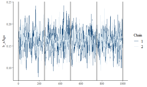
cmdstanr works with several packages in the Stan ecosystem, including posterior and bayesplot.
# draws for bayesplot
draws <- posterior::as_draws_array(fit_m2)

# trace plot
bayesplot::mcmc_trace(x = draws, pars = "b_zAge") +
geom_vline(xintercept = seq(0, 1000, 250),
           alpha = 0.25,
           size = 2)
This vertical lines are placed at each checkpoint.
Model Comparison
These models can then be compared with approximate leave-one-out
cross-validation (via the R package loo).
loo_compare(loo(fit_m1), loo(fit_m2))

#>       elpd_diff se_diff
#> fit_m1    0.0       0.0
#> fit_m2 -203.6      65.4
Compare to brm
For a sanity check, here is fit_m2 fitted with
brms. The estimates should be (basically) the same.
fit_brms <- brm(
  formula = bf(formula = count ~ zAge + zBase,
               family = poisson()),
  data = epilepsy,
  chains = 2,
  iter = 2000
)

fit_brms

#>  Family: poisson
#>   Links: mu = log
#> Formula: count ~ zAge + zBase
#>    Data: epilepsy (Number of observations: 236)
#>   Draws: 2 chains, each with iter = 2000; warmup = 1000; thin = 1;
#>          total post-warmup draws = 2000
#>
#> Population-Level Effects:
#>           Estimate Est.Error l-95% CI u-95% CI Rhat Bulk_ESS Tail_ESS
#> Intercept     1.84      0.03     1.78     1.89 1.00     1247     1310
#> zAge          0.16      0.02     0.11     0.21 1.00     1226     1191
#> zBase         0.60      0.01     0.57     0.63 1.00     1107     1229
#>
#> Draws were sampled using sampling(NUTS). For each parameter, Bulk_ESS
#> and Tail_ESS are effective sample size measures, and Rhat is the potential
#> scale reduction factor on split chains (at convergence, Rhat = 1).
The results for the parameter estimates and diagnostics are very similar (as expected).
Example 3: User Defined Priors
chkpt_brms() includes ... which passes any
number of (valid) arguments to brm(). Accordingly, priors
can be specified as though brm() was used.
path <- create_folder(folder_name = "chkpt_folder_m3")

# priors
bprior <- prior(constant(1), class = "b") +
  prior(constant(2), class = "b", coef = "zBase") +
  prior(constant(0.5), class = "sd")

# fit model
fit_m3 <- chkpt_brms(
  bf(formula = count ~ zAge + zBase  + (1 | patient),
     family = poisson()),
  prior = bprior,
  data = epilepsy,
  path  = path,
  iter_warmup = 1000,
  iter_sampling = 1000,
  iter_per_chkpt = 250,
  brmsfit = TRUE
)
prior_summary() can be used to confirm that the priors
found their way into the model correctly, i.e.,
prior_summary(fit_m3)

#>                   prior     class      coef   group resp dpar nlpar bound       source
#>             constant(1)         b                                                 user
#>             constant(1)         b      zAge                               (vectorized)
#>             constant(2)         b     zBase                                       user
#>  student_t(3, 1.4, 2.5) Intercept                                              default
#>           constant(0.5)        sd                                                 user
#>           constant(0.5)        sd           patient                       (vectorized)
#>           constant(0.5)        sd Intercept patient                       (vectorized)