MCMC Diagnostics
Donny Williams
5/20/2020
Source:vignettes/mcmc_diagnostics.Rmd
mcmc_diagnostics.RmdIntroduction
The algorithms in BGGM are based on Gibbs samplers. In the context of covariance matrix estimation, as opposed, to, say, hierarchical models, this allows for efficiently sampling the posterior distribution. Furthermore, in all samplers the empirical covariance matrix is used as the starting value which reduces the length of the burn-in (or warm-up). Still yet it is important to monitor convergence. See here for an introduction to MCMC diagnostics.
R packages
# need the developmental version
if (!requireNamespace("remotes")) {
  install.packages("remotes")
}

# install from github
remotes::install_github("donaldRwilliams/BGGM")
library(BGGM)
ACF plot
This first example includes an “acf” plot that looks at the auto correlation of the samples. In general, we do not want the samples to be strongly correlated or related to the previous samples (or lags ). I am not sure there are general guidelines, but typically we do not want “auto correlation…for higher values of k, [because] this indicates a high degree of correlation between our samples and slow mixing” source
Here is an example for ordinal data.
# data
Y <- ptsd[,1:10]

# fit model
# + 1 makes first category a 1
fit <- estimate(Y + 1, type = "ordinal")
To check the convergence of a partial correlation, we need the parameter name. These are printed as follows
convergence(fit, print_names = TRUE)

#>  [1] "B1--B2"         "B1--B3"         "B2--B3"         "B1--B4"         "B2--B4"         "B3--B4"         "B1--B5"
#>  [8] "B2--B5"         "B3--B5"         "B4--B5"         "B1--C1"         "B2--C1"         "B3--C1"         "B4--C1"
#> [15] "B5--C1"         "B1--C2"         "B2--C2"         "B3--C2"         "B4--C2"         "B5--C2"         "C1--C2"
#> [22] "B1--D1"         "B2--D1"         "B3--D1"         "B4--D1"         "B5--D1"         "C1--D1"         "C2--D1"
#> [29] "B1--D2"         "B2--D2"         "B3--D2"         "B4--D2"         "B5--D2"         "C1--D2"         "C2--D2"
#> [36] "D1--D2"         "B1--D3"         "B2--D3"         "B3--D3"         "B4--D3"         "B5--D3"         "C1--D3"
#> [43] "C2--D3"         "D1--D3"         "D2--D3"         "B1_(Intercept)" "B2_(Intercept)" "B3_(Intercept)" "B4_(Intercept)"
#> [50] "B5_(Intercept)" "C1_(Intercept)" "C2_(Intercept)" "D1_(Intercept)" "D2_(Intercept)" "D3_(Intercept)"
Note the (Intercept) which reflect the fact that the
ordinal approach is a multivariate probit model with only
intercepts.
The next step is to make the plot
convergence(fit, param = "B1--B2", type = "acf")
The argument param can take any number of parameters and
a plot will be made for each (e.g..,
param = c("B1--B2", B1--B3)). In this case, the auto
correlations looks acceptable and actually really good (note the drop to
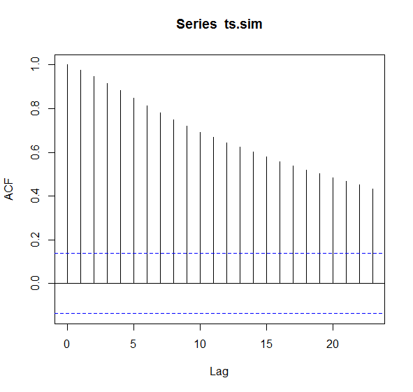
zero). A problematic acf plot would have the black lines
start at 1.0 and perhaps never go below
0.20.
To make this clear, I simulated time series data taking the code from here

This would be considered problematic. If this occurs, one solution could be to thin the samples manually
# extract samples
samps <- fit$post_samp$pcors

# iterations
iter <- fit$iter

# thinning interval
thin <-  5

# save every 5th (add 50 which is the burnin)
new_iter <- length(seq(1,to = iter + 50 , by = thin))

# replace (add 50 which is the burnin)
fit$post_samp$pcors <- samps[,,seq(1,to = iter + 50, by = thin)]

# replace iter
fit$iter <- new_iter - 50

# check thinned
convergence(fit, param = "B1--B2", type = "acf")
or perhaps just running the model for more iterations (e.g.,
increasing iter in estimate). The above is
quite convoluted but note convergence should not typically be an issue.
And it might come in handy to know that the samples can be replaced and
the other functions in BGGM will still work with the
object fit.
Trace plot
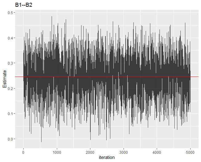
The next example is a trace plot. Here we are looking for good “mixing”.
convergence(fit, param = "B1--B2", type = "trace")
Admittedly the term “mixing” is vague. But in general the plot should look like this example, where there is no place that the chain is “stuck”. See here for problematic trace plots.