⚠️ Project Has Moved ⚠️
BGGM is now maintained at https://github.com/rast-lab/BGGM.
This original repository (https://github.com/donaldRwilliams/BGGM) is no longer actively developed. All new issues, pull requests, and development take place at:
👉 https://github.com/rast-lab/BGGM
Please update your links accordingly.
The R package BGGM provides tools for making Bayesian inference in Gaussian graphical models (GGM, Williams and Mulder 2020). The methods are organized around two general approaches for Bayesian inference: (1) estimation and (2) hypothesis testing. The key distinction is that the former focuses on either the posterior or posterior predictive distribution (Gelman et al. 1996; see section 5 in Rubin 1984), whereas the latter focuses on model comparison with the Bayes factor (Jeffreys 1961; Kass and Raftery 1995).
Installation
To install the latest release version (2.1.1) from CRAN use
The current developmental version can be installed with
if (!requireNamespace("remotes")) {
  install.packages("remotes")
}
remotes::install_github("rast-lab/BGGM")
Dealing with Errors
There are automatic checks for BGGM. However, that only checks for Linux and BGGM is built on Windows. The most common installation errors occur on OSX. An evolving guide to address these issues is provided in the Troubleshoot Section.
Overview
The methods in BGGM build upon existing algorithms that are well-known in the literature. The central contribution of BGGM is to extend those approaches:
-
Bayesian estimation with the novel matrix-F prior distribution (Mulder and Pericchi 2018)
- Estimation (Williams 2018)
-
Bayesian hypothesis testing with the matrix-F prior distribution (Williams and Mulder 2019)
-
Comparing Gaussian graphical models (Williams 2018; Williams et al.
-
Extending inference beyond the conditional (in)dependence structure (Williams 2018)
Posterior uncertainty intervals for the partial correlations
The computationally intensive tasks are written in c++ via the R package Rcpp (Eddelbuettel et al. 2011) and the c++ library Armadillo (Sanderson and Curtin 2016). The Bayes factors are computed with the R package BFpack (Mulder et al. 2019). Furthermore, there are plotting functions for each method, control variables can be included in the model (e.g., ~ gender), and there is support for missing values (see bggm_missing).
Supported Data Types
Continuous: The continuous method was described in Williams (2018). Note that this is based on the customary Wishart distribution.
Binary: The binary method builds directly upon Talhouk et al. (2012) that, in turn, built upon the approaches of Lawrence et al. (2008) and Webb and Forster (2008) (to name a few).
Ordinal: The ordinal methods require sampling thresholds. There are two approach included in BGGM. The customary approach described in Albert and Chib (1993) (the default) and the ‘Cowles’ algorithm described in Cowles (1996).
Mixed: The mixed data (a combination of discrete and continuous) method was introduced in Hoff (2007). This is a semi-parametric copula model (i.e., a copula GGM) based on the ranked likelihood. Note that this can be used for only ordinal data (not restricted to “mixed” data).
Illustrative Examples
There are several examples in the Vignettes section.
Basic Usage
It is common to have some combination of continuous and discrete (e.g., ordinal, binary, etc.) variables. BGGM (as of version 2.0.0) can readily be used for these kinds of data. In this example, a model is fitted for the gss data in BGGM.
Visualize
The data are first visualized with the psych package, which readily shows the data are “mixed”.
# dev version
library(BGGM)
library(psych)

# data
Y <- gss

# histogram for each node
psych::multi.hist(Y, density = FALSE)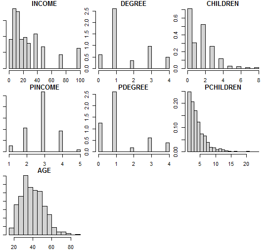
Fit Model
A Gaussian copula graphical model is estimated as follows
type can be continuous, binary, ordinal, or mixed. Note that type is a misnomer, as the data can consist of only ordinal variables (for example).
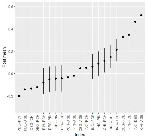
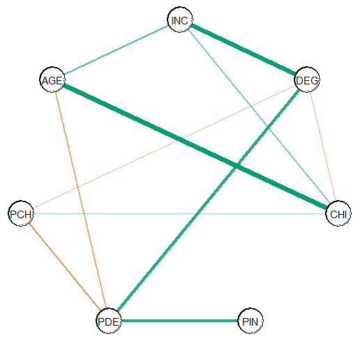
Summarize Relations
The estimated relations are summarized with
summary(fit)

#> BGGM: Bayesian Gaussian Graphical Models
#> ---
#> Type: mixed
#> Analytic: FALSE
#> Formula:
#> Posterior Samples: 5000
#> Observations (n): 464
#> Nodes (p): 7
#> Relations: 21
#> ---
#> Call:
#> estimate(Y = Y, type = "mixed")
#> ---
#> Estimates:
#>  Relation Post.mean Post.sd Cred.lb Cred.ub
#>  INC--DEG     0.463   0.042   0.377   0.544
#>  INC--CHI     0.148   0.053   0.047   0.251
#>  DEG--CHI    -0.133   0.058  -0.244  -0.018
#>  INC--PIN     0.087   0.054  -0.019   0.196
#>  DEG--PIN    -0.050   0.058  -0.165   0.062
#>  CHI--PIN    -0.045   0.057  -0.155   0.067
#>  INC--PDE     0.061   0.057  -0.050   0.175
#>  DEG--PDE     0.326   0.056   0.221   0.438
#>  CHI--PDE    -0.043   0.062  -0.162   0.078
#>  PIN--PDE     0.345   0.059   0.239   0.468
#>  INC--PCH     0.052   0.052  -0.052   0.150
#>  DEG--PCH    -0.121   0.056  -0.228  -0.012
#>  CHI--PCH     0.113   0.056   0.007   0.224
#>  PIN--PCH    -0.080   0.059  -0.185   0.052
#>  PDE--PCH    -0.200   0.058  -0.305  -0.082
#>  INC--AGE     0.211   0.050   0.107   0.306
#>  DEG--AGE     0.046   0.055  -0.061   0.156
#>  CHI--AGE     0.522   0.039   0.442   0.594
#>  PIN--AGE    -0.020   0.054  -0.122   0.085
#>  PDE--AGE    -0.141   0.057  -0.251  -0.030
#>  PCH--AGE    -0.033   0.051  -0.132   0.063
#> ---
The summary can also be plotted
References
Albert, James H, and Siddhartha Chib. 1993. “Bayesian Analysis of Binary and Polychotomous Response Data.” Journal of the American Statistical Association 88 (422): 669–79.
Cowles, Mary Kathryn. 1996. “Accelerating Monte Carlo Markov Chain Convergence for Cumulative-Link Generalized Linear Models.” Statistics and Computing 6 (2): 101–11. https://doi.org/10.1007/bf00162520.
Eddelbuettel, Dirk, Romain François, J Allaire, et al. 2011. “Rcpp: Seamless r and c++ Integration.” Journal of Statistical Software 40 (8): 1–18.
Gelman, Andrew, Xiao-Li Meng, and Hal Stern. 1996. “Posterior Predictive Assessment of Model Fitness via Realized Discrepancies.” Statistica Sinica 6 (4): 733–807.
Hoff, Peter D. 2007. “Extending the Rank Likelihood for Semiparametric Copula Estimation.” The Annals of Applied Statistics 1 (1): 265–83. https://doi.org/10.1214/07-AOAS107.
Jeffreys, Harold. 1961. The theory of probability. Oxford University Press.
Kass, Robert E, and Adrian E Raftery. 1995. “Bayes Factors.” Journal of the American Statistical Association 90 (430): 773–95.
Lawrence, Earl, Derek Bingham, Chuanhai Liu, and Vijayan N Nair. 2008. “Bayesian Inference for Multivariate Ordinal Data Using Parameter Expansion.” Technometrics 50 (2): 182–91.
Mulder, Joris, Xin Gu, Anton Olsson-Collentine, et al. 2019. “BFpack: Flexible Bayes Factor Testing of Scientific Theories in r.” arXiv Preprint arXiv:1911.07728.
Mulder, Joris, and Luis Pericchi. 2018. “The Matrix-F Prior for Estimating and Testing Covariance Matrices.” Bayesian Analysis, no. 4: 1–22. https://doi.org/10.1214/17-BA1092.
Rubin, Donald B. 1984. “Bayesianly Justifiable and Relevant Frequency Calculations for the Applied Statistician.” The Annals of Statistics, 1151–72. https://doi.org/10.1214/aos/1176346785.
Sanderson, Conrad, and Ryan Curtin. 2016. “Armadillo: A Template-Based c++ Library for Linear Algebra.” Journal of Open Source Software 1 (2): 26. https://doi.org/10.21105/joss.00026.
Talhouk, Aline, Arnaud Doucet, and Kevin Murphy. 2012. “Efficient Bayesian Inference for Multivariate Probit Models with Sparse Inverse Correlation Matrices.” Journal of Computational and Graphical Statistics 21 (3): 739–57.
Webb, Emily L, and Jonathan J Forster. 2008. “Bayesian Model Determination for Multivariate Ordinal and Binary Data.” Computational Statistics & Data Analysis 52 (5): 2632–49. https://doi.org/10.1016/j.csda.2007.09.008.
Williams, Donald R. 2018. “Bayesian Estimation for Gaussian Graphical Models: Structure Learning, Predictability, and Network Comparisons.” arXiv, ahead of print. https://doi.org/10.31234/OSF.IO/X8DPR.
Williams, Donald R, and Joris Mulder. 2019. “Bayesian Hypothesis Testing for Gaussian Graphical Models: Conditional Independence and Order Constraints.” PsyArXiv, ahead of print. https://doi.org/10.31234/osf.io/ypxd8.
Williams, Donald R, and Joris Mulder. 2020. “BGGM: Bayesian Gaussian Graphical Models in r.” PsyArXiv.
Williams, Donald R, Philippe Rast, Luis R Pericchi, and Joris Mulder. 2020. “Comparing Gaussian Graphical Models with the Posterior Predictive Distribution and Bayesian Model Selection.” Psychological Methods, ahead of print. https://doi.org/10.1037/met0000254.