Custom Network Comparisons

Background

It is quite common to have partial correlation networks (GGMs) for various subgroups, say, males and females, a control and treatment group, or perhaps several educational levels. In this case, it is important to not only determine whether the groups are different, but actually compare the groups in a way that answers a specific question of interest.

To date, most R packages provide a few ways to compare groups, including BGGM (version 1.0.0). In version 2.0.0, however, BGGM includes a new feature for the function ggm_compare_ppc that enables users to compare networks in any way they want.

Basic Idea

The technical details of the approach are described in (Williams et al. 2020). The basic idea is to

Draw samples from the posterior distribution, assuming the groups are equal (i.e., the “null” model).
Generate the posterior predictive distribution for the chosen test-statistic (how the groups are being compared)
- This can be understood as what we would expect to observe in the future (e.g., in replication), assuming the groups were in fact equal.
Compute the test-statistic for the observed groups.
Then compare the observed test-statistic to the predictive distribution (what is expected under the “null” model).
- If the observed error is larger than the model assuming group equality, this suggests that the groups are different.

In BGGM, the default is to compare the groups with respect to (symmetric) Kullback-Leibler divergence (i.e., “distance” between multivariate normal distributions) and the sum of squared error (for the partial correlation matrix). This was shown to be quite powerful in Williams et al. (2020), while also having a low false positive rate.

In the following, the focus is on defining custom functions and using them with ggm_compare_ppc. In all examples, post-traumatic stress disorder networks are compared (Fried et al. 2018).

R packages

# need the developmental version
if (!requireNamespace("remotes")) { 
  install.packages("remotes")   
}   

# install from github
remotes::install_github("donaldRwilliams/BGGM")

Data

Only the correlation matrices are available. Hence, multivariate normal data is generated with that exact correlation structure via the R package MASS.

# need these packages
library(BGGM)
library(ggplot2)
library(assortnet)
library(networktools)
library(MASS)

# group 1
Yg1 <- MASS::mvrnorm(n = 926, 
                     mu = rep(0, 16), 
                     Sigma = ptsd_cor3, 
                     empirical = TRUE)

# group 2
Yg2 <- MASS::mvrnorm(n = 956, 
                     mu = rep(0, 16), 
                     Sigma = ptsd_cor4, 
                     empirical = TRUE)

Illustrative Examples

Correlation

This first example looks at the correlation between partial correlations of the two networks. Note that it could be two networks have what is considered a large correlation. However, the question here is, assuming the groups are equal, just how large should the correlation be? This is needed to interpret the observed test-statistic.

Step 1: Define Custom Function

The first step is to define a custom function that takes two data matrices and the output is the chosen test-statistic (in this case a correlation)

f <- function(Yg1, Yg2){
  # number of nodes
  p <- ncol(Yg1)
  
  # index of off-diagonal
  indices <- upper.tri( diag(p))
  
  # group 1:
  # fit model
  g1_fit <- estimate(Yg1, analytic = TRUE)
  # pcors
  g1_pcors <- pcor_mat(g1_fit)[indices]
  
  # group 2
  # fit model
  g2_fit <- estimate(Yg2, analytic = TRUE)
  # pcors
  g2_pcors <- pcor_mat(g2_fit)[indices]
  
  # test-statistic
  cor(g1_pcors, g2_pcors)
  }

Step 2: Compute the Observed Score

The next step is to compute the observed test-statistic, that is, the correlation between the partial correlations.

obs <- f(Yg1, Yg2)

# observed
obs

## [1] 0.5399268

Step 3: Predictive Check

With the function, f, and the observed scores, obs, in hand, what is left is the predictive check

ppc <- BGGM::ggm_compare_ppc(Yg1, Yg2, 
                       FUN = f, 
                       custom_obs = obs, 
                       iter = 1000, 
                       loss = FALSE)

Note that loss = FALSE controls how the p-value is computed. It is an indicator of whether the test-statistic is a “loss” (a bad thing). In this case, a large correlation is a good thing so it is set to FALSE. The results can then be printed

ppc

## BGGM: Bayesian Gaussian Graphical Models 
## --- 
## Test: Global Predictive Check 
## Posterior Samples: 1000 
##   Group 1: 926 
##   Group 2: 956 
## Nodes:  16 
## Relations: 120 
## --- 
## Call: 
## BGGM::ggm_compare_ppc(Yg1, Yg2, iter = 1000, FUN = f, custom_obs = obs, 
##     loss = FALSE)
## --- 
## Custom: 
##  
##    contrast custom.obs p.value
##  Yg1 vs Yg2       0.54       0
## ---

which shows the posterior predictive p-value is zero. This indicates that the observed correlation is lower than the entire predictive distribution (the distribution of correlations for future data, assuming group equality)

and finally plot the results

plot(ppc)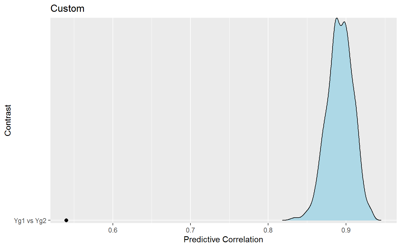

The density is the predictive distribution for the correlation. Recall that this is the correlation that we would expect, given the groups were actually the same, and the black point is the observed correlation. In this case, it seems quite clear that the “null model” is inadequate–the groups are apparently quite different.

Hamming Distance

The next example is Hamming distance, which, in this case, is the squared error for the adjacency matrices. It seems reasonable to think of this as a test for different network structures or patterns of zeros and ones.

Step 1: Define Custom Function

The first step is to define a custom function that takes two data matrices and the output is the chosen test-statistic (in this case Hamming distance)

f <- function(Yg1, Yg2){
  # nodes
  p <- ncol(Yg1)
  
  # index of off-diagonal
  indices <- upper.tri( diag(p))

  # fit models
  fit1 <-  BGGM::estimate(Yg1, analytic = TRUE)
  fit2 <-  BGGM::estimate(Yg2, analytic = TRUE)
  
  # select graphs
  sel1 <- BGGM::select(fit1)
  sel2 <- BGGM::select(fit2)
  
  # hamming distance
  sum((sel1$adj[indices] - sel2$adj[indices]) ^ 2)
}

Step 2: Compute the Observed Score

The next step is to compute the observed test-statistic, that is, the Hamming distance between adjacency matrices

obs <- f(Yg1, Yg2)

# observed
obs

## [1] 60

Step 3: Predictive Check

With the function, f, and the observed scores, obs, in hand, what is left is the predictive check

ppc <- BGGM::ggm_compare_ppc(Yg1, Yg2, 
                       FUN = f, 
                       custom_obs = obs, 
                       iter = 1000)

The results can then be printed

ppc

## BGGM: Bayesian Gaussian Graphical Models 
## --- 
## Test: Global Predictive Check 
## Posterior Samples: 1000 
##   Group 1: 926 
##   Group 2: 956 
## Nodes:  16 
## Relations: 120 
## --- 
## Call: 
## BGGM::ggm_compare_ppc(Yg1, Yg2, iter = 1000, FUN = f, custom_obs = obs)
## --- 
## Custom: 
##  
##    contrast custom.obs p.value
##  Yg1 vs Yg2         60       0
## ---

And then plot the results

plot(ppc)

## $plot_custom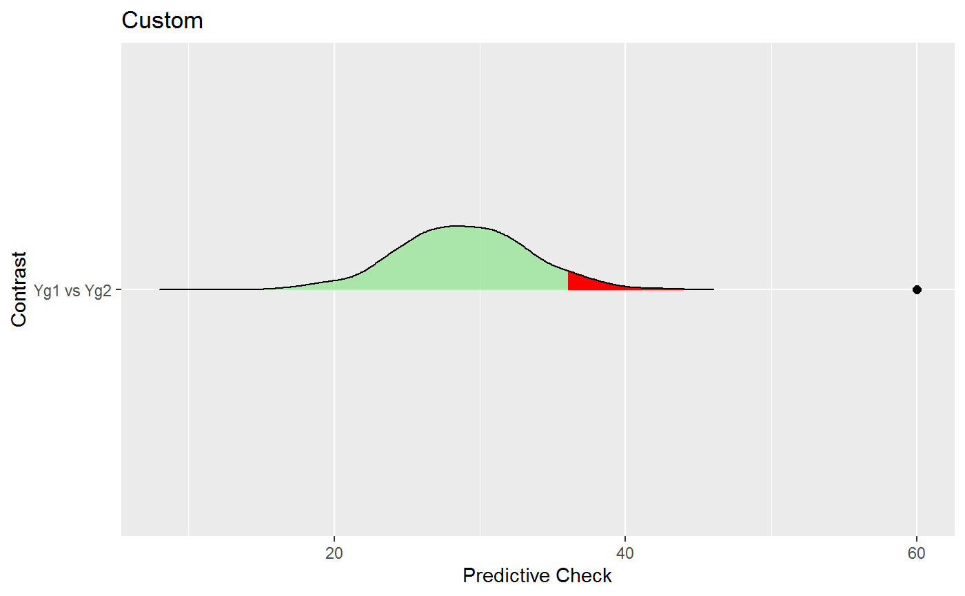

This result is intriguing. Whereas the correlation looked at the relation between partial correlation, here there seems to be evidence that the adjacency matrices are different (perhaps suggesting that the conditional independence structure is different).

Partial Correlation Matrix Distance

There might also be interest in the so-called correlation matrix distance (Herdin et al. 2005). This is also easily tested, in this case for the partial correlation matrix.

Step 1: Define Custom Function

f <- function(Yg1, Yg2){
  # nodes
  p <- ncol(Yg1)
  
  # index of off-diagonal
  indices <- upper.tri( diag(p))

  # fit models
  fit1 <-  BGGM::estimate(Yg1, analytic = TRUE)
  fit2 <-  BGGM::estimate(Yg2, analytic = TRUE)
  
  pcor1 <- BGGM::pcor_mat(fit1) 
  pcor2 <- BGGM::pcor_mat(fit2)
  
  # CDM for partial correlations
  # note: numerator is the trace; denominator is the Frobenius norm
  1 - (sum(diag(pcor1 %*% pcor2)) / (norm(pcor1, type = "f") * norm(pcor2, type = "f")))
}

Step 2: Compute the Observed Score

The next step is to compute the observed test-statistic, that is, the Partial Correlation Matrix Distance

obs <- f(Yg1, Yg2)

# observed
obs

## [1] 0.3430489

Step 3: Predictive Check

With the function, f, and the observed scores, obs, in hand, what is left is the predictive check

ppc <- BGGM::ggm_compare_ppc(Yg1, Yg2, 
                       FUN = f, 
                       custom_obs = obs, 
                       iter = 1000)

The results can then be printed

ppc

## BGGM: Bayesian Gaussian Graphical Models 
## --- 
## Test: Global Predictive Check 
## Posterior Samples: 1000 
##   Group 1: 926 
##   Group 2: 956 
## Nodes:  16 
## Relations: 120 
## --- 
## Call: 
## BGGM::ggm_compare_ppc(Yg1, Yg2, iter = 1000, FUN = f, custom_obs = obs)
## --- 
## Custom: 
##  
##    contrast custom.obs p.value
##  Yg1 vs Yg2      0.343       0
## ---

which again provides a p-value of zero.

Note that the object ppc includes the predictive samples that allows for user defined plots (in the event something custom is desired).

hist(ppc$predictive_custom, 
     xlim = c(0, obs), 
     main = "Partial Correlation Matrix Distance")
abline(v = obs)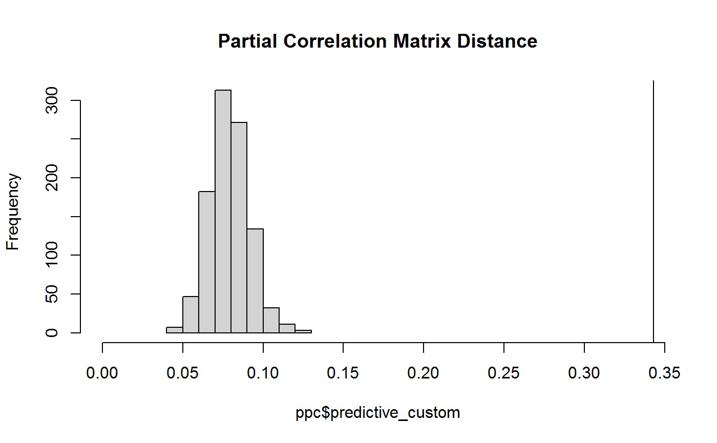

Note that the line is the observed which again makes it clear that the distance is quite surprising, assuming the null model were true.

Assortment

This next example is assortment (Newman 2003), which is a measure related to clustering in a network. Here the test is for a difference in assortment. This is computed by taking the difference (absolute value) for each draw from the predictive distribution.

Step 1: Define Custom Function

# clusters based on DSM-5
comms <- c(
  rep("A", 4),
  rep("B", 7),
  rep("C", 5)
)

f <- function(Yg1, Yg2){

  fit1 <-  BGGM::estimate(Yg1, analytic = TRUE)
  fit2 <-  BGGM::estimate(Yg2, analytic = TRUE)

  pcor1 <- BGGM::pcor_mat(fit1)
  pcor2 <- BGGM::pcor_mat(fit2)

  assort1 <- assortnet::assortment.discrete(pcor1, types = comms,
                                         weighted = TRUE,
                                         SE = FALSE, M = 1)$r

  assort2 <- assortnet::assortment.discrete(pcor2, types = comms,
                                          weighted = TRUE,
                                          SE = FALSE, M = 1)$r
  (assort1 - assort2)
}

Step 2: Compute the Observed Score

The next step is to compute the observed test-statistic, that is, assortment for the two groups

obs <- f(Yg1, Yg2)

# observed
obs

## [1] 0.1915766

Step 3: Predictive Check

With the function, f, and the observed score, obs, in hand, the next step is the predictive check

ppc <- BGGM::ggm_compare_ppc(Yg1, Yg2, 
                       FUN = f, 
                       custom_obs = obs, 
                       iter = 1000)

The results can then be printed

ppc

## BGGM: Bayesian Gaussian Graphical Models 
## --- 
## Test: Global Predictive Check 
## Posterior Samples: 1000 
##   Group 1: 926 
##   Group 2: 956 
## Nodes:  16 
## Relations: 120 
## --- 
## Call: 
## BGGM::ggm_compare_ppc(Yg1, Yg2, iter = 1000, FUN = f, custom_obs = obs)
## --- 
## Custom: 
##  
##    contrast custom.obs p.value
##  Yg1 vs Yg2      0.192       0
## ---

and plotted

plot(ppc)

## $plot_custom

## Picking joint bandwidth of 0.00663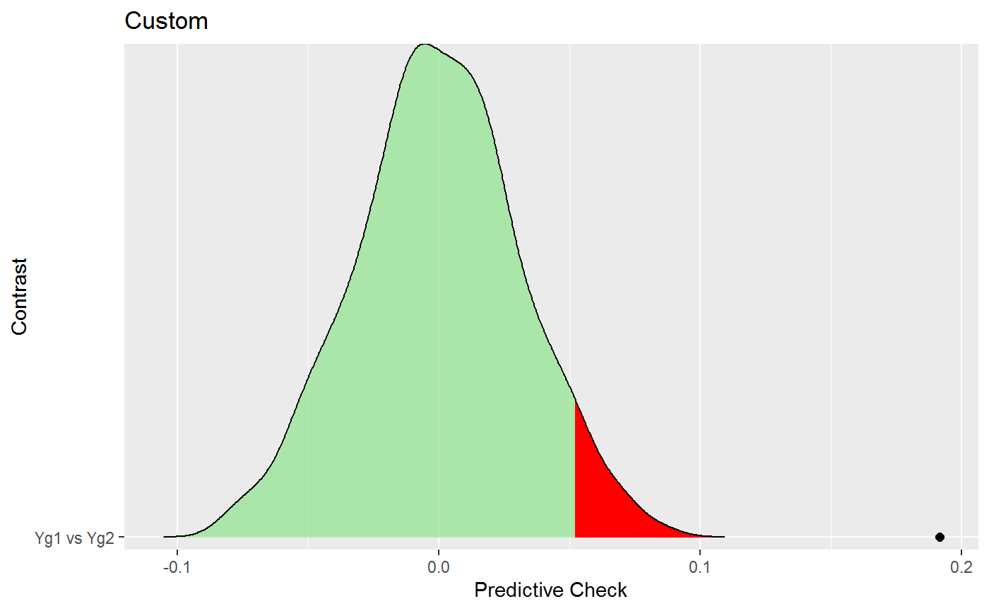

which shows that the clustering in the data appears to be different (given the observed value exceeds the entire predictive distribution).

Expected Influence

This last example looks at the expected influence for the network (Robinaugh, Millner, and McNally 2016). In this case, the sum of squared error is the test statistic. This is computed from the squared error for each draw from the predictive distribution.

Step 1: Define Custom Function

f <- function(Yg1, Yg2){

  fit1 <-  BGGM::estimate(Yg1, analytic = TRUE)
  fit2 <-  BGGM::estimate(Yg2, analytic = TRUE)

  pcor1 <- BGGM::pcor_mat(fit1)
  pcor2 <- BGGM::pcor_mat(fit2)

  ei1 <- networktools::expectedInf(pcor1)$step1
 
  ei2 <- networktools::expectedInf(pcor2)$step1
   sum((ei1 - ei2)^2)
}

Step 2: Compute the Observed Score

The next step is to compute the observed test-statistic, that is, the sum of squared error for expected influence

obs <- f(Yg1, Yg2)

# observed
obs

## [1] 0.518462

Step 3: Predictive Check

With the function, f, and the observed scores, obs, in hand, what is left is the predictive check

ppc <- BGGM:::ggm_compare_ppc(Yg1, Yg2, 
                       FUN = f, 
                       custom_obs = obs, 
                       iter = 1000)

The results can then be printed

ppc

## BGGM: Bayesian Gaussian Graphical Models 
## --- 
## Test: Global Predictive Check 
## Posterior Samples: 1000 
##   Group 1: 926 
##   Group 2: 956 
## Nodes:  16 
## Relations: 120 
## --- 
## Call: 
## BGGM:::ggm_compare_ppc(Yg1, Yg2, iter = 1000, FUN = f, custom_obs = obs)
## --- 
## Custom: 
##  
##    contrast custom.obs p.value
##  Yg1 vs Yg2      0.518       0
## ---

and plotted

hist(ppc$predictive_custom, 
    xlim = c(0, obs),
     main = "Expected Influence\n Sum of Squared Error")
abline(v = obs)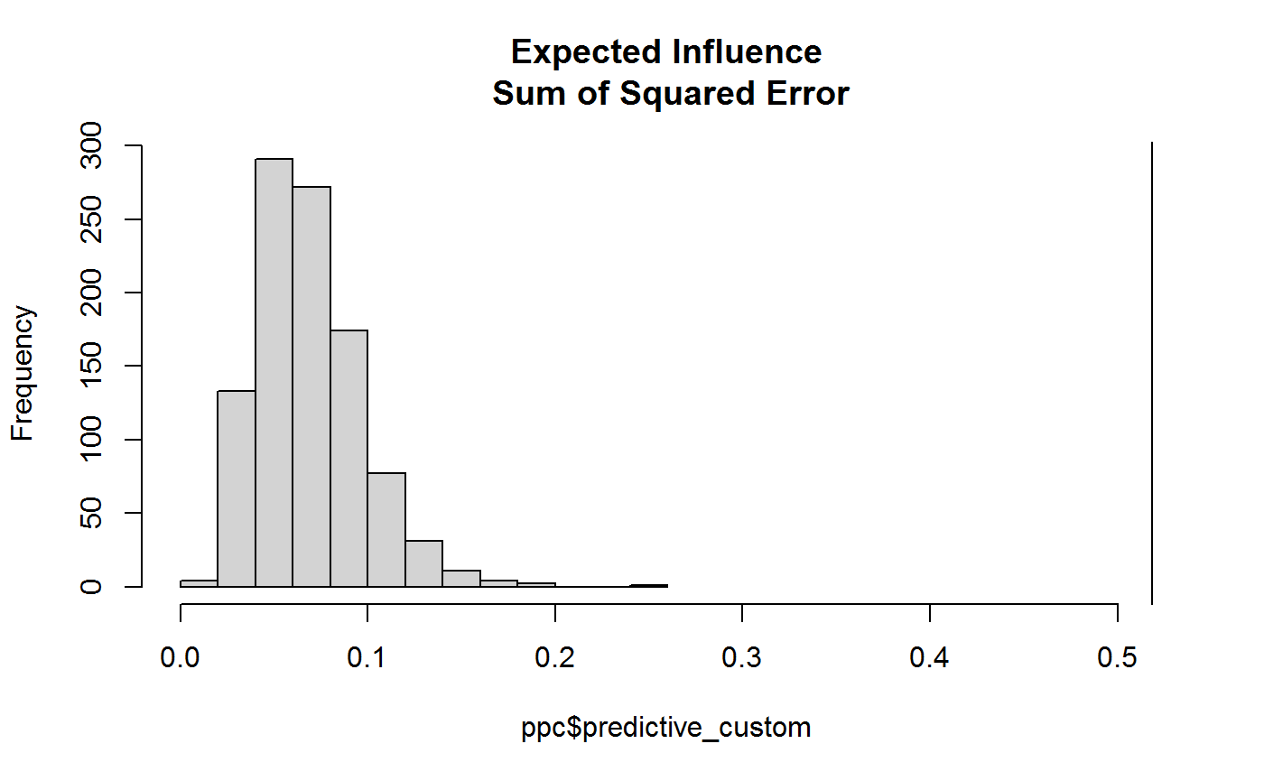

which again shows the sum of squared error for expected influence far exceeds what would be expected, assuming the null model were true.

Two Notes of Caution

Note that only the default in BGGM have been shown to have nominal error rates. However, there is a proof that suggests the error rate cannot be larger than $2\alpha$ (Meng et al. 1994), and, further, a predictive check is typically below $\alpha$ (i.e., a tendency to be conservative, Gelman et al. 2013).
Failing to reject the null model does not indicate the groups are the same! To test for equality see ggm_compare_explore and ggm_compare_confirm.

Conclusion

These example certainly open the door for tailoring network comparison to answer specific research questions.

References

Fried, Eiko I, Marloes B Eidhof, Sabina Palic, Giulio Costantini, Hilde M Huisman-van Dijk, Claudi LH Bockting, Iris Engelhard, Cherie Armour, Anni BS Nielsen, and Karen-Inge Karstoft. 2018. “Replicability and Generalizability of Posttraumatic Stress Disorder (PTSD) Networks: A Cross-Cultural Multisite Study of PTSD Symptoms in Four Trauma Patient Samples.” Clinical Psychological Science 6 (3): 335–51.

Gelman, Andrew et al. 2013. “Two Simple Examples for Understanding Posterior p-Values Whose Distributions Are Far from Uniform.” Electronic Journal of Statistics 7: 2595–2602. https://doi.org/10.1214/13-ejs854.

Herdin, Markus, Nicolai Czink, Hüseyin Ozcelik, and Ernst Bonek. 2005. “Correlation Matrix Distance, a Meaningful Measure for Evaluation of Non-Stationary MIMO Channels.” In 2005 IEEE 61st Vehicular Technology Conference, 1:136–40. IEEE. https://doi.org/10.1109/vetecs.2005.1543265.

Meng, Xiao-Li et al. 1994. “Posterior Predictive

p

-Values.” The Annals of Statistics 22 (3): 1142–60.

Newman, Mark EJ. 2003. “Mixing Patterns in Networks.” Physical Review E 67 (2): 026126.

Robinaugh, Donald J, Alexander J Millner, and Richard J McNally. 2016. “Identifying Highly Influential Nodes in the Complicated Grief Network.” Journal of Abnormal Psychology 125 (6): 747.

Williams, Donald R, Philippe Rast, Luis R Pericchi, and Joris Mulder. 2020. “Comparing Gaussian Graphical Models with the Posterior Predictive Distribution and Bayesian Model Selection.” Psychological Methods. https://doi.org/10.1037/met0000254.

Donny Williams

5/19/2020

Background

Basic Idea

R packages

Data

Illustrative Examples

Correlation

Step 1: Define Custom Function

Step 2: Compute the Observed Score

Step 3: Predictive Check

Hamming Distance

Step 1: Define Custom Function

Step 2: Compute the Observed Score

Step 3: Predictive Check

Partial Correlation Matrix Distance

Step 1: Define Custom Function

Step 2: Compute the Observed Score

Step 3: Predictive Check

Assortment

Step 1: Define Custom Function

Step 2: Compute the Observed Score

Step 3: Predictive Check

Expected Influence

Step 1: Define Custom Function

Step 2: Compute the Observed Score

Step 3: Predictive Check

Two Notes of Caution

Conclusion

References