Multivariate Normal Imputation

Impute values, assuming a multivariate normal distribution, with the posterior predictive distribution. For binary, ordinal, and mixed (a combination of discrete and continuous) data, the values are first imputed for the latent data and then converted to the original scale.

mvn_imputation(
  Y,
  type = "continuous",
  iter = 1000,
  progress = TRUE,
  save_all = FALSE
)

Arguments

Y	Matrix (or data frame) of dimensions n (observations) by p (variables).
type	Character string. Which type of data for Y ? The options include continuous, binary, ordinal, or mixed. Note that mixed can be used for data with only ordinal variables. See the note for further details.
iter	Number of iterations (posterior samples; defaults to 1000).
progress	Logical. Should a progress bar be included (defaults to TRUE) ?
save_all	Logical. Should each imputed dataset be stored (defaults to FALSE which saves the imputed missing values) ?

Value

An object of class mvn_imputation:

• Y The last imputed dataset.

• ppd_missing A matrix of dimensions iter by the number of missing values.

• ppd_mean A vector including the means of the posterior predictive distribution for the missing values.

• Y_all An 3D array with iter matrices of dimensions n by p (NULL when save_all = FALSE).

Details

Missing values are imputed with the approach described in Hoff (2009) . The basic idea is to impute the missing values with the respective posterior pedictive distribution, given the observed data, as the model is being estimated. Note that the default is TRUE, but this ignored when there are no missing values. If set to FALSE, and there are missing values, list-wise deletion is performed with na.omit.

References

Hoff PD (2009). A first course in Bayesian statistical methods, volume 580. Springer.

Examples

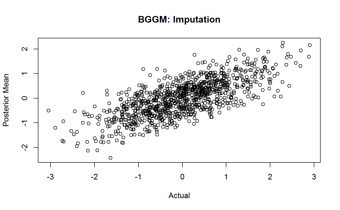
# \donttest{
# obs
n <- 5000

# n missing
n_missing <- 1000

# variables
p <- 16

# data
Y <- MASS::mvrnorm(n, rep(0, p), ptsd_cor1)

# for checking
Ymain <- Y

# all possible indices
indices <- which(matrix(0, n, p) == 0,
                 arr.ind = TRUE)

# random sample of 1000 missing values
na_indices <- indices[sample(5:nrow(indices),
                             size = n_missing,
                             replace = FALSE),]

# fill with NA
Y[na_indices] <- NA

# missing = 1
Y_miss <- ifelse(is.na(Y), 1, 0)

# true values (to check)
true <- unlist(sapply(1:p, function(x)
        Ymain[which(Y_miss[,x] == 1),x] ))

# impute
fit_missing <- mvn_imputation(Y, progress = FALSE, iter = 250)

print(fit_missing, n_rows = 20)
#> BGGM: Bayesian Gaussian Graphical Models 
#> --- 
#> Multivariate Normal Imputation
#> --- 
#> Estimates:
#> 
#>    Value Post.mean Post.sd Cred.lb Cred.ub
#>    57--1     1.937   0.493   0.849   2.878
#>   244--1    -0.401   0.501  -1.390   0.581
#>   273--1    -0.437   0.502  -1.388   0.538
#>   317--1    -0.014   0.515  -0.983   0.965
#>   403--1     0.939   0.509  -0.002   1.913
#>   449--1    -1.502   0.507  -2.377  -0.455
#>   461--1    -0.144   0.525  -1.146   0.914
#>   556--1     0.709   0.508  -0.293   1.591
#>   558--1    -0.525   0.513  -1.647   0.470
#>   686--1    -2.127   0.489  -3.044  -1.172
#>   777--1     0.707   0.514  -0.298   1.655
#>   824--1    -0.273   0.480  -1.191   0.565
#>   872--1    -0.707   0.557  -1.806   0.354
#>   908--1    -1.073   0.550  -2.259  -0.067
#>   948--1    -0.187   0.510  -1.107   0.871
#>   958--1     0.448   0.539  -0.546   1.492
#>  1026--1    -1.336   0.576  -2.443  -0.211
#>  1074--1     0.063   0.542  -1.019   1.062
#>  1116--1     0.222   0.536  -0.757   1.265
#>  1139--1    -1.627   0.483  -2.570  -0.668


# plot
plot(x =  true,
     y = fit_missing$ppd_mean,
     main = "BGGM: Imputation",
     xlab = "Actual",
     ylab = "Posterior Mean")
# }