Partial Correlation Sum — pcor

Compute and test partial correlation sums either within or between GGMs (e.g., different groups), resulting in a posterior distribution.

Usage

pcor_sum(..., iter = NULL, relations)

Arguments

...: An object of class estimate. This can be either one or two fitted objects.
iter: Number of iterations (posterior samples; defaults to the number in the object).
relations: Character string. Which partial correlations should be summed?

Value

An object of class posterior_sum, including the sum and possibly the difference for two sums.

Details

Some care must be taken when writing the string for partial_sum. Below are several examples

Just a Sum: Perhaps a sum is of interest, and not necessarily the difference of two sums. This can be written as

partial_sum <- c("A1--A2 + A1--A3 + A1--A4")

which will sum those relations.

Comparing Sums: When comparing sums, each must be seperated by ";". For example,

partial_sum <- c("A1--A2 + A1--A3; A1--A2 + A1--A4")

which will sum both and compute the difference. Note that there cannot be more than two sums, such that c("A1--A2 + A1--A3; A1--A2 + A1--A4; A1--A2 + A1--A5") will result in an error.

Comparing Groups:

When more than one fitted object is suppled to object it is assumed that the groups should be compared for the same sum. Hence, in this case, only the sum needs to be written.

partial_sum <- c("A1--A2 + A1--A3 + A1--A4")

The above results in that sum being computed for each group and then compared.

Examples

# \donttest{
# data
Y <- bfi

# males
Y_males <- subset(Y, gender == 1, select = -c(education, gender))[,1:5]

# females
Y_females <- subset(Y, gender == 2, select = -c(education, gender))[,1:5]

# males
fit_males <- estimate(Y_males, seed = 1,
                      progress = FALSE)

# fit females
fit_females <- estimate(Y_females, seed = 2,
                        progress = FALSE)


sums <- pcor_sum(fit_males,
                 fit_females,
                 relations = "A1--A2 + A1--A3")
# print
sums
#> BGGM: Bayesian Gaussian Graphical Models 
#> --- 
#> Network Stats: Posterior Sum
#> Posterior Samples: 5000 
#> --- 
#> Estimates 
#> 
#> Sum: 
#>                   Post.mean Post.sd Cred.lb Cred.ub
#> g1: A1--A2+A1--A3    -0.314   0.039  -0.392  -0.239
#> g2: A1--A2+A1--A3    -0.344   0.026  -0.394  -0.293
#> --- 
#> 
#> Difference:
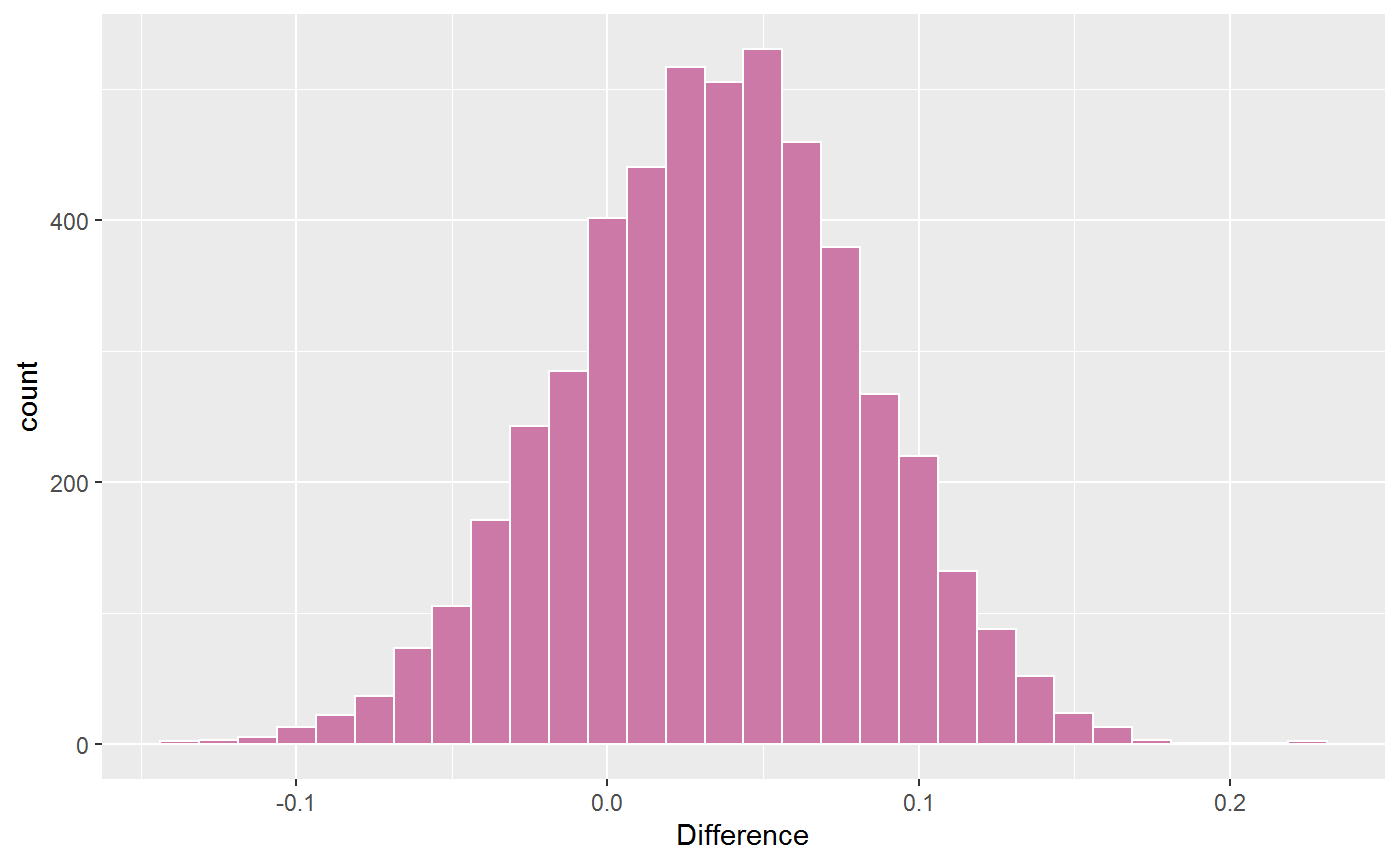
#> g1: A1--A2+A1--A3 - g2: A1--A2+A1--A3 
#> 
#>  Post.mean Post.sd Cred.lb Cred.ub Prob.greater Prob.less
#>       0.03   0.047  -0.062   0.123        0.742     0.258
#> --- 

# plot difference
plot(sums)[[3]]
#> `stat_bin()` using `bins = 30`. Pick better value with `binwidth`.

# }