Plot summary.ggm_compare_estimate Objects
Source: R/ggm_compare_estimate.default.R
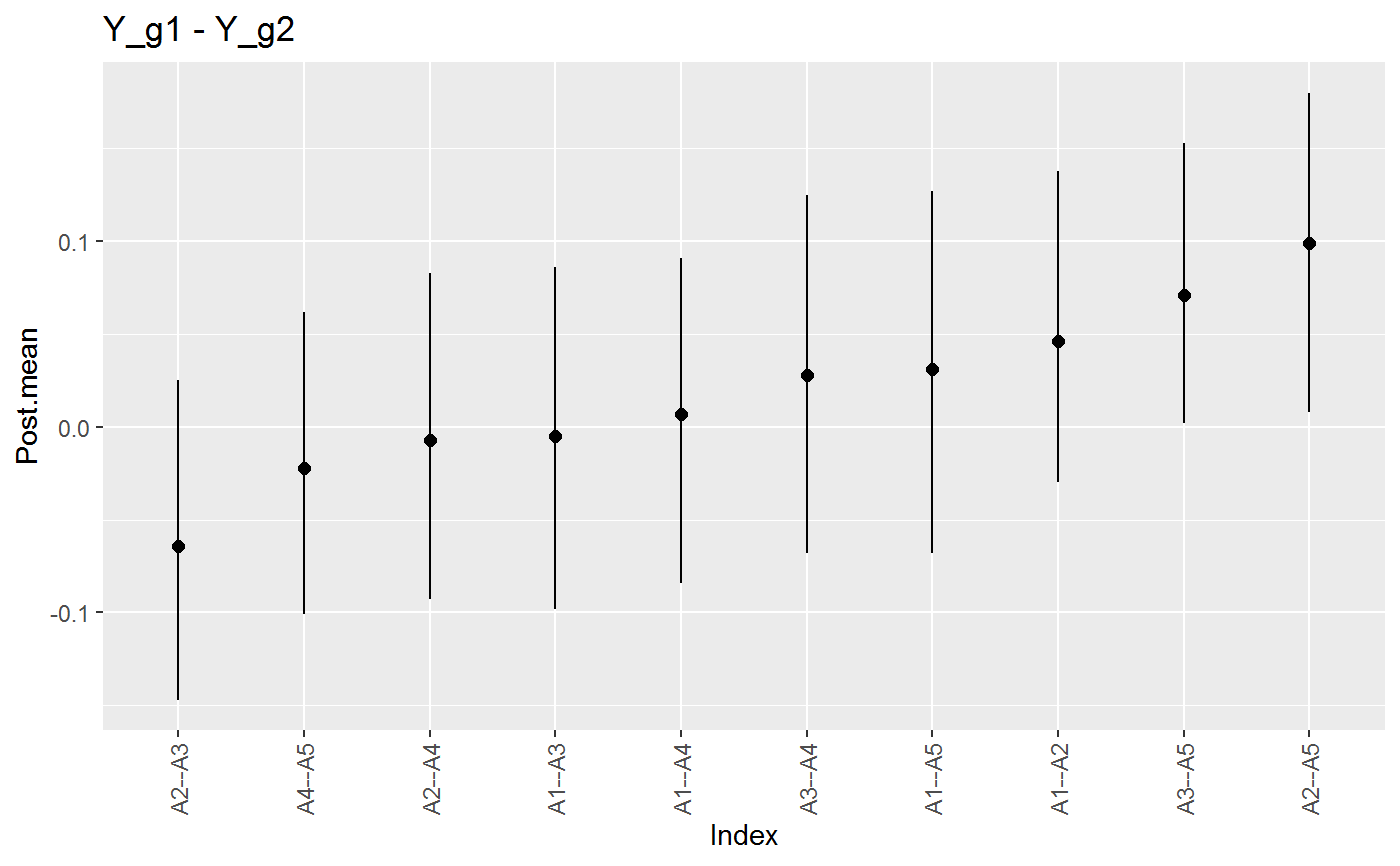
plot.summary.ggm_compare_estimate.RdVisualize the posterior distribution differences.
Usage
# S3 method for class 'summary.ggm_compare_estimate'
plot(x, color = "black", size = 2, width = 0, ...)Examples
# \donttest{
# note: iter = 250 for demonstrative purposes
# data
Y <- bfi[complete.cases(bfi),]

# males and females
Ymale <- subset(Y, gender == 1,
                select = -c(gender,
                            education))[,1:10]

Yfemale <- subset(Y, gender == 2,
                  select = -c(gender,
                              education))[,1:10]

# fit model
fit <- ggm_compare_estimate(Ymale,  Yfemale,
                            type = "ordinal",
                            iter = 250,
                            prior_sd = 0.25,
                            progress = FALSE)
#> Warning: imputation during model fitting is
#> currently only implemented for 'continuous' data.
#> Warning: imputation during model fitting is
#> currently only implemented for 'continuous' and 'mixed' data.
#> Warning: imputation during model fitting is
#> currently only implemented for 'continuous' and 'mixed' data.

plot(summary(fit))
#> [[1]]

#>
# }
#>
# }