Introduction

GGMncv is set up for low-dimensional settings, that is, when the number of observations (\(n\)) is much greater than the number of nodes (\(p\)). This is perhaps not typical in the Gaussian graphical modeling literature, and is a direct result of my (the author of GGMncv) field encountering low-dimensional data most often (see for example Williams et al. 2019; Williams and Rast 2020). As a result, the defaults are honed in for low-dimensional data!

Of course, GGMncv can readily be used for high-dimensional data. In what follows, I highlight several issues that may arise, in addition to solutions to overcome those issues.

Failure Altogether

By default, GGMncv uses the sample based (inverse) covariance matrix for the initial values, which is needed for employing nonconvex regularization. When \(p > n\), GGMncv will produce an error because the sample based (inverse) covariance matrix cannot be inverted in this situation.

For example, notice the error when running the following code:

library(GGMncv)

# p > n
set.seed(2)
main <- gen_net(p = 50, 
                edge_prob = 0.05)

set.seed(2)
y <- MASS::mvrnorm(n = 49, 
                   mu = rep(0, 50), 
                   Sigma = main$cors)

fit <- ggmncv(cor(y), n = nrow(y))
#> Error in solve.default(R): system is computationally singular: reciprocal condition number = 3.39775e-18

Solution

The solution is to provide an function for the initial matrix. To this end, GGMncv includes the function lediot_wolf which is a shrinkage estimator (Ledoit and Wolf 2004). It is important to note that any function can be used, so long as it return the inverse correlation matrix.

fit <- ggmncv(cor(y), n = nrow(y), 
              penalty = "atan",
              progress = FALSE,
              initial = ledoit_wolf, Y = y)

Notice the Y = y, which is used internally to pass additional arguments via ... to the function provided in initial.

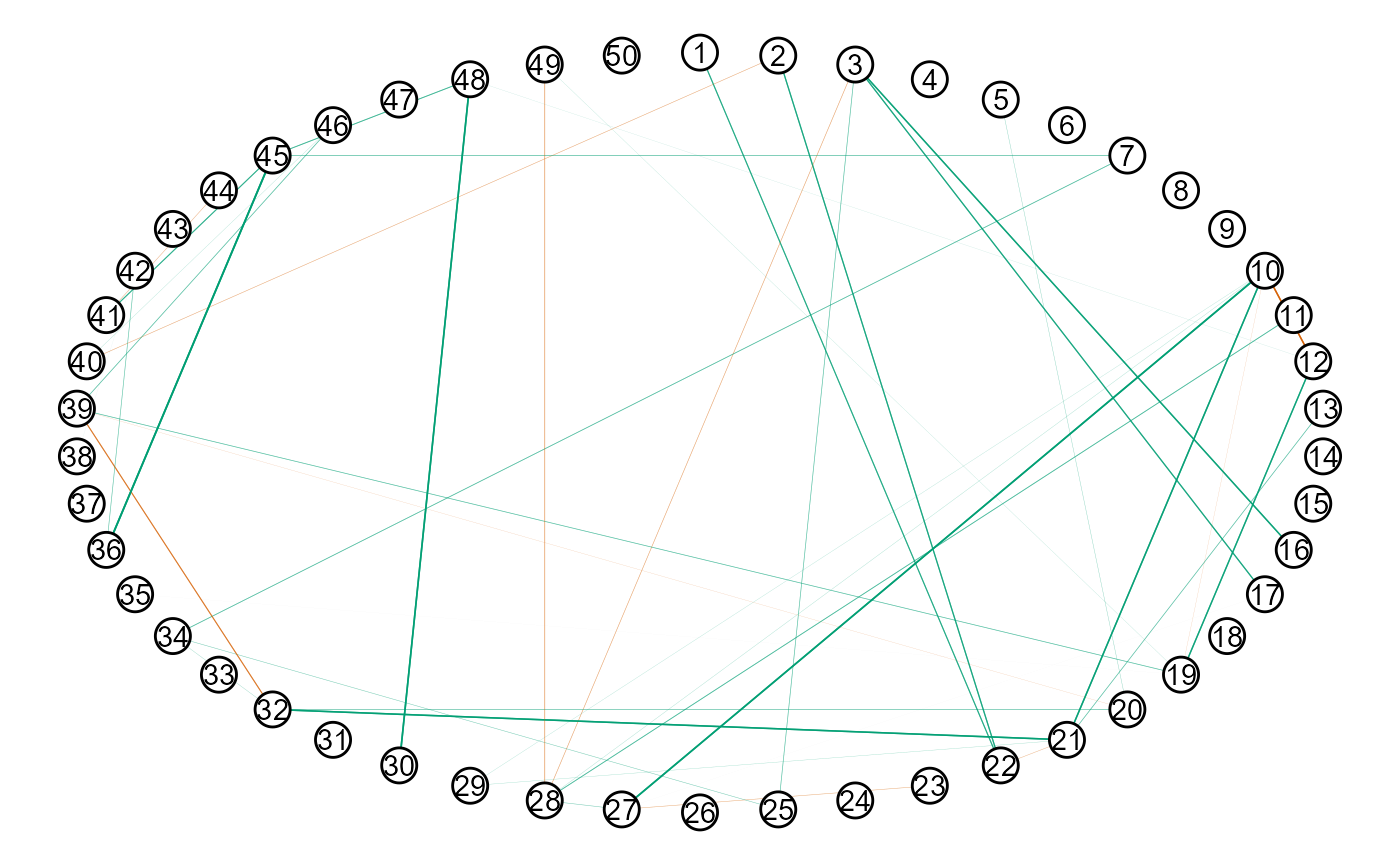
The conditional dependence structure can then be plotted with

plot(get_graph(fit), 
     node_size = 5)

Here is an example of providing a function.

initial_ggmncv <- function(y, ...){
  Rinv <- corpcor::invcor.shrink(y, verbose = FALSE)
  return(Rinv)
}

fit2 <- ggmncv(cor(y), n = nrow(y), 
               penalty = "atan",
               progress = FALSE,
               initial = initial_ggmncv, 
               y = y)

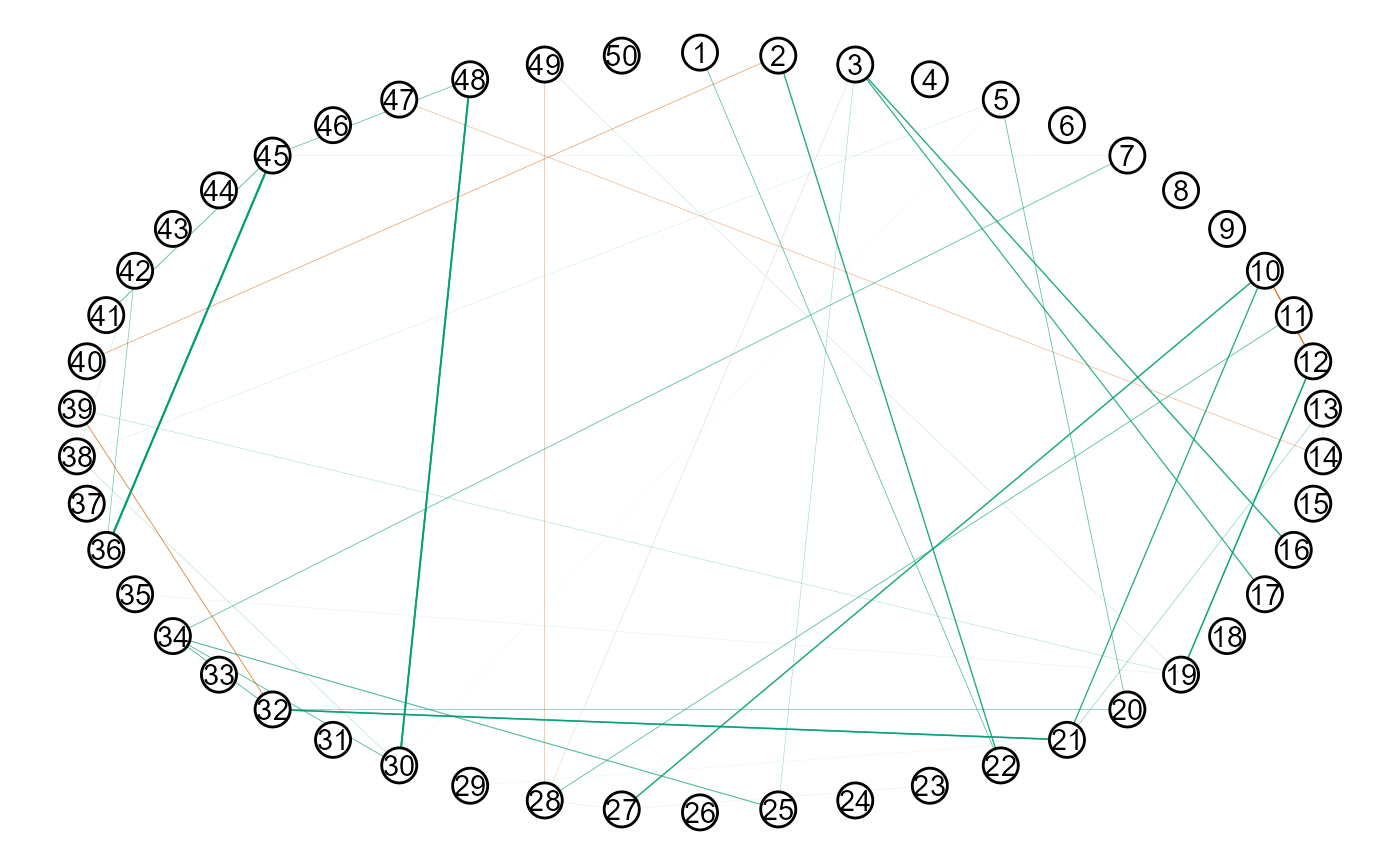
plot(get_graph(fit2), 
     node_size = 5)

Perhaps it is of interest to compare performance, given that different initial values were used.

# ledoit and wolf
score_binary(estimate = fit$adj, 
             true = main$adj, 
             model_name = "lw")
#>       measure     score model_name
#> 1 specificity 0.9750859         lw
#> 2 sensitivity 0.2459016         lw
#> 3   precision 0.3409091         lw
#> 4      recall 0.2459016         lw
#> 5    f1_score 0.2857143         lw
#> 6         mcc 0.2583199         lw

# Shaffer and strimmer
score_binary(estimate = fit2$adj, 
             true = main$adj,  
             model_name = "ss")
#>       measure     score model_name
#> 1 specificity 0.9759450         ss
#> 2 sensitivity 0.2459016         ss
#> 3   precision 0.3488372         ss
#> 4      recall 0.2459016         ss
#> 5    f1_score 0.2884615         ss
#> 6         mcc 0.2622113         ss

Works but Bad Performance

Perhaps a trickier situation is when the covariance matrix can be inverted, but it is still ill-conditioned. This can occur when \(p\) approaches but does not exceed \(n\). Here performance can be very bad.

# p -> n
main <- gen_net(p = 50, 
                edge_prob = 0.05)

y <- MASS::mvrnorm(n = 60, 
                   mu = rep(0, 50), 
                   Sigma = main$cors)

fit <- ggmncv(cor(y), n = nrow(y), 
              penalty = "atan",
              progress = FALSE)

score_binary(estimate = fit$adj, 
             true = main$adj)
#>       measure       score
#> 1 specificity  0.07302405
#> 2 sensitivity  0.88524590
#> 3   precision  0.04766108
#> 4      recall  0.88524590
#> 5    f1_score  0.09045226
#> 6         mcc -0.03444145

This is extremely problematic because there was no error, and the performance was terrible (note: 1 - specificity = the false positive rate).

Solution

One solution is again to provide a function to initial.

fit <- ggmncv(cor(y), n = nrow(y), 
              progress = FALSE,
              penalty = "atan",
              initial = ledoit_wolf, Y = y)

score_binary(estimate = fit$adj, 
             true = main$adj)
#>       measure     score
#> 1 specificity 0.9725086
#> 2 sensitivity 0.2622951
#> 3   precision 0.3333333
#> 4      recall 0.2622951
#> 5    f1_score 0.2935780
#> 6         mcc 0.2632312

An additional solution is to use \(L_1\)-regularization, i.e.,

fit_l1 <- ggmncv(cor(y), n = nrow(y), 
              progress = FALSE, 
              penalty = "lasso")

score_binary(estimate = fit_l1$adj, 
             true = main$adj)
#>       measure     score
#> 1 specificity 0.9914089
#> 2 sensitivity 0.1311475
#> 3   precision 0.4444444
#> 4      recall 0.1311475
#> 5    f1_score 0.2025316
#> 6         mcc 0.2215582

A quick comparison of KL-divergence

# atan
kl_mvn(true = solve(main$cors), estimate = fit$Theta)
#> [1] 1.539283

# lasso
kl_mvn(true = solve(main$cors), estimate = fit_l1$Theta)
#> [1] 2.374752

References

Ledoit, Olivier, and Michael Wolf. 2004. “A Well-Conditioned Estimator for Large-Dimensional Covariance Matrices.” Journal of Multivariate Analysis 88 (2): 365–411.

Williams, Donald R, and Philippe Rast. 2020. “Back to the Basics: Rethinking Partial Correlation Network Methodology.” British Journal of Mathematical and Statistical Psychology 73 (2): 187–212.

Williams, Donald R, Mijke Rhemtulla, Anna C Wysocki, and Philippe Rast. 2019. “On Nonregularized Estimation of Psychological Networks.” Multivariate Behavioral Research 54 (5): 719–50.

High Dimensional Data: Must Read!!

Introduction

Failure Altogether

Solution

Works but Bad Performance

Solution

References