Introduction

For some research questions, there might be expectations in regards to the directions of the edges. For example, in symptom networks, all relations are often hypothesized to be positive (i.e., positive manifold). In turn, any negative relations are thought to be spurious.

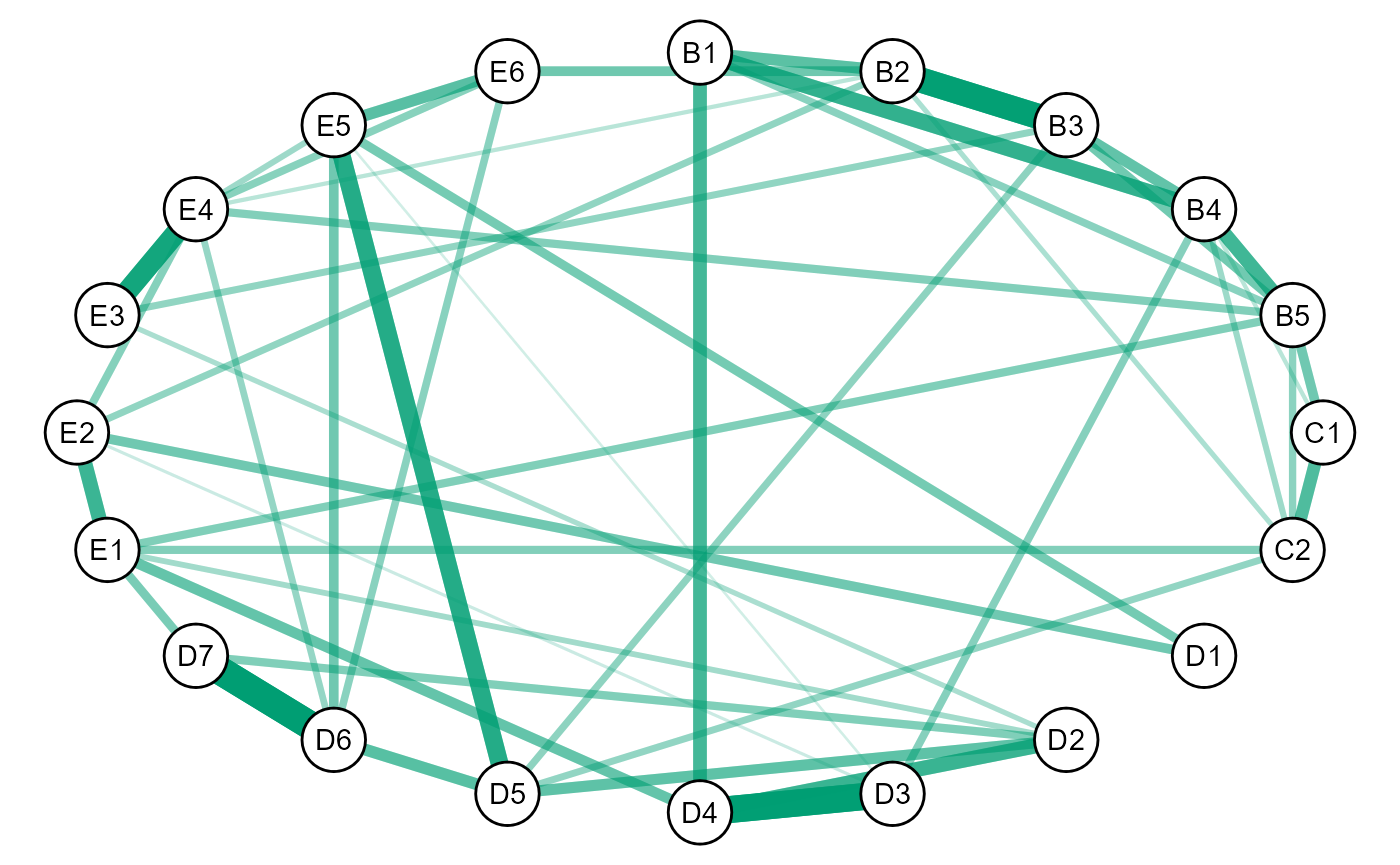
In GGMncv, it is possible to estimate the conditional dependence structure, given that all edges in the graph are positive (sign restriction).

Packages

library(GGMncv)
library(corrplot)

Correlations

The ptsd dataset includes 20 post-traumatic stress symptoms. The following visualizes the correlation matrix:

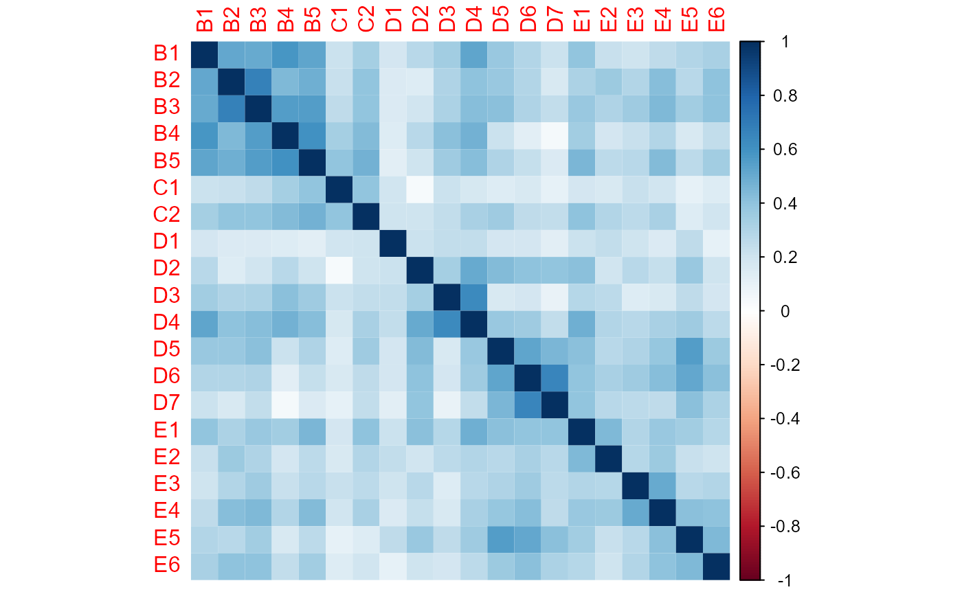
corrplot::corrplot(cor(ptsd), method = "shade")

Notice that all of the correlations are positive.

Partial Correlations

Here are the partial correlations:

pcors <- -cov2cor(solve(cor(ptsd))) + diag(ncol(ptsd))

corrplot::corrplot(pcors, 
                   method = "shade")

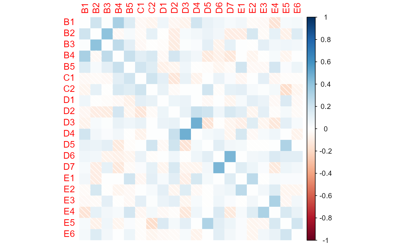
Notice that some relations went to essentially zero (white), whereas other changed direction altogether.

GGM

Here the conditional dependence structure is selected via ggmncv:

# fit model
fit <- GGMncv::ggmncv(cor(ptsd),
                      n = nrow(ptsd),
                      progress = FALSE,
                      penalty = "atan")

# plot graph
plot(GGMncv::get_graph(fit),
     edge_magnify = 10,
     node_names = colnames(ptsd))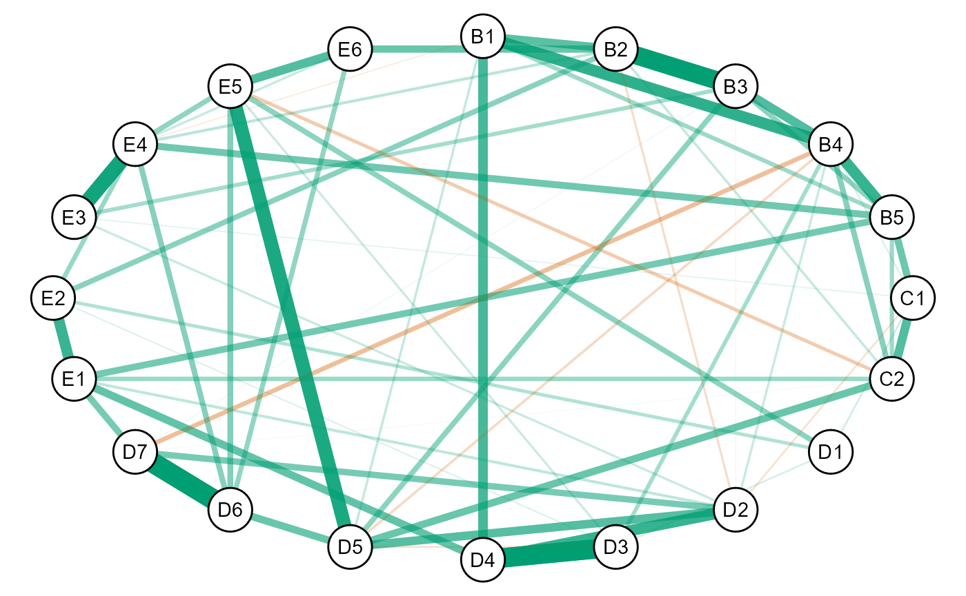

Notice a few negatives are included in the graph.

Sign Restriction

Here the graph is re-estimated, with the constraint that all of negative edges in the above plot are actually zero.

# set negatives to zero (sign restriction)
adj_new <- ifelse(fit$P <= 0, 0, 1)

check_zeros <- TRUE

# track trys
iter <- 0

# iterate until all positive
while(check_zeros){
  iter <- iter + 1
  fit_new <- GGMncv::constrained(cor(ptsd), adj = adj_new)
  check_zeros <- any(fit_new$wadj < 0)
  adj_new <- ifelse(fit_new$wadj <= 0, 0, 1)
}

# make graph object
new_graph <- list(P = fit_new$wadj,
                  adj = adj_new)
class(new_graph) <- "graph"

# plot graph
plot(new_graph,
     edge_magnify = 10,
     node_names = colnames(ptsd))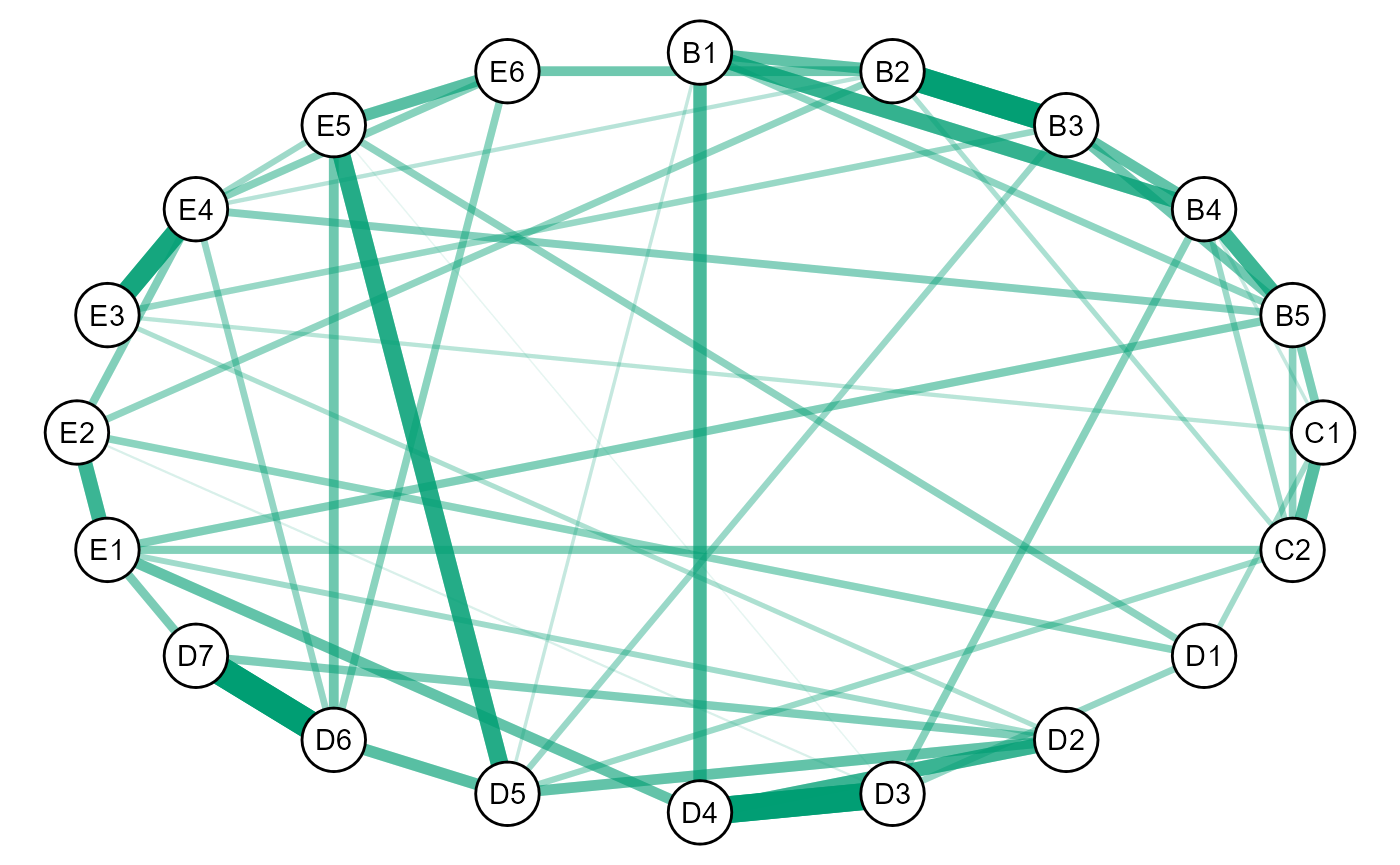

The graph now only includes positive edges. Note this is not the same as simply removing the negative relations, as, in this case, this is the maximum likelihood estimate for the inverse covariance matrix.

Note also new_graph is making the graph class so that it can be plotted with plot.

Alternative Approach

The above essentially takes the selected graph, and then re-estimates it with the constraint that the negative edges are zero. Perhaps a more sophisticated approach is to select the graph with those constraints.

This can be implemented with:

R <- cor(ptsd)
n <- nrow(ptsd)
p <- ncol(ptsd)

# store fitted models
fit <- ggmncv(R = R, 
              n = n, 
              progress = FALSE, 
              store = TRUE, 
              n_lambda = 50)

# all fitted models
# sol: solution
sol_path <- fit$fitted_models

# storage
bics <- NA
Thetas <- list()

for(i in seq_along(sol_path)){
  
  # positive in wi is a negative partial
  adj_new <- ifelse(sol_path[[i]]$wi >= 0, 0, 1)
  
  check_zeros <- TRUE
  
  # track trys
  iter <- 0
  
  # iterate until all positive
  while(check_zeros){
    iter <- iter + 1
    fit_new <- GGMncv::constrained(R, adj = adj_new)
    check_zeros <- any(fit_new$wadj < 0)
    adj_new <- ifelse(fit_new$wadj <= 0, 0, 1)
}
  
  bics[i] <- GGMncv:::gic_helper(
    Theta = fit_new$Theta,
    R = R,
    n = n,
    p = p,
    type = "bic",
    edges = sum(fit_new$Theta[upper.tri(fit_new$Theta)] != 0)
  )
  
  Thetas[[i]] <- fit_new$Theta
}

# select via minimizing bic
# (then convert to partial correlatons)
pcors <- -(cov2cor(Thetas[[which.min(bics)]]) - diag(p))

# make graph class
new_graph <- list(P = pcors,
                  adj = ifelse(pcors == 0, 0, 1))
class(new_graph) <- "graph"

# plot graph
plot(new_graph,
     edge_magnify = 10,
     node_names = colnames(ptsd))