Three Ways to Test the Same Hypothesis

Introduction

On a Facebook methods group, there was a question about testing hypotheses in networks. In the comments, it was suggested that BGGM could be used to test the hypothesis. And it turns out that BGGM really shines for testing expectations (see for example Rodriguez et al. 2020).

In this vignette, I demonstrate three ways to go about testing the same hypothesis, which is essentially testing for a difference in the sum of partial correlations between groups.

R package

# need the developmental version
if (!requireNamespace("remotes")) { 
  install.packages("remotes")   
}   

# install from github
remotes::install_github("donaldRwilliams/BGGM")
library(BGGM)

Data

For demonstrative purposes, I use the bfi data and test the hypotheses in males and females

# data
Y <- bfi

# males
Y_males <- subset(Y, gender == 1, select = -c(education, gender))[,1:5]

# females
Y_females <- subset(Y, gender == 2, select = -c(education, gender))[,1:5]

Approach 1: Posterior Difference

The first approach is rather straightforward, with the caveat that the method needs to be implemented by the user. Note that I could certainly implement this in BGGM, assuming there is enough interest. Please make a feature request here.

Hypothesis

The hypothesis was that a sum of relations was larger in one group, for example,

$\begin{align} \mathcal{H}_0: (\rho^{male}_{A1--A2}\; + \; \rho^{male}_{A1--A3}) = (\rho^{female}_{A1--A2}\; + \; \rho^{female}_{A1--A3}) \\ \mathcal{H}_1: (\rho^{male}_{A1--A2}\; + \; \rho^{male}_{A1--A3}) > (\rho^{female}_{A1--A2}\; + \; \rho^{female}_{A1--A3}) \end{align}$ Note that the hypothesis is related to the sum of relations, which is readily tested in BGGM.

Fit Models

The first step is to estimate the model for each group

# fit female
fit_female <- estimate(Y_females, seed = 2)

# fit males
fit_male <- estimate(Y_males, seed = 1)

For an example, I used the default which is to assume the data is Gaussian. This can be changed with type = either binary, ordinal, or mixed.

Extract the Samples

The next step is to extract the posterior samples for each relation

post_male <- posterior_samples(fit_male)[,c("A1--A2", "A1--A3")]

post_female <- posterior_samples(fit_female)[,c("A1--A2", "A1--A3")]

Note that the column names reflect the upper-triangular elements of the partial correlation matrix. Hence, the first name (e.g.,A1) must be located before the second name (e.g., A2) in the data matrix. This can be understood in reference to the column numbers: 1--2 is correct whereas 2--1 will result in an error.

Sum and Compute Difference

The next step is to sum the relations and compute the difference

# sum males
sum_male <- rowSums(post_male) 

# sum females
sum_female <- rowSums(post_female)

# difference
diff <- sum_male - sum_female

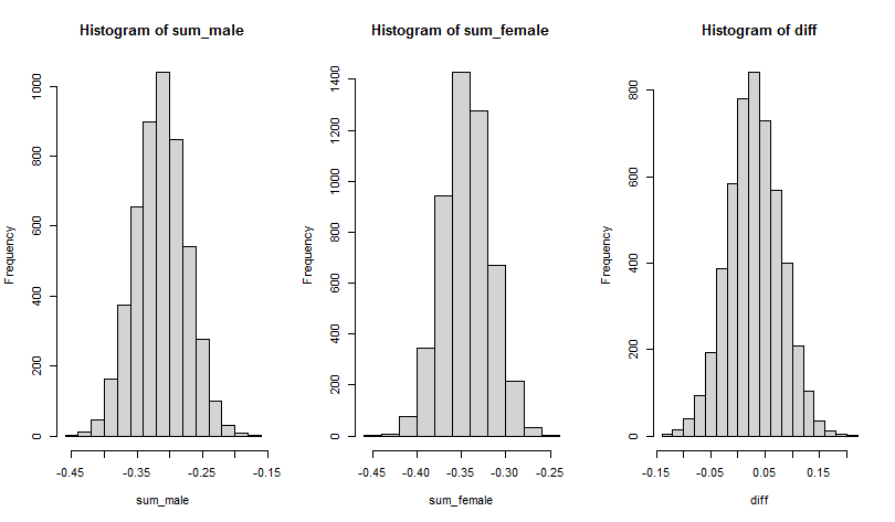
which can then be plotted

# three column
par(mfrow=c(1,3))

# male sum
hist(sum_male)

# female sum
hist(sum_female)

# difference
hist(diff)

Posterior Probability

Next compute the posterior probability the sum is larger in males than females

# posterior prob
mean(sum_male > sum_female)

#> 0.737

and then the credible interval for the difference

quantile(diff, probs = c(0.025, 0.975))

#>        2.5%       97.5% 
#> -0.06498586  0.12481253

Approach 2: Predictive Check

The next approach is based on a posterior predictive check. The hypothesis is essentially the same as above, but for the predictive distribution, that is,

$\begin{align} \mathcal{H}_0: (\rho^{male^{yrep}}_{A1--A2}\; + \; \rho^{male^{yrep}}_{A1--A3}) = (\rho^{female^{yrep}}_{A1--A2}\; + \; \rho^{female^{yrep}}_{A1--A3}) \\ \mathcal{H}_1: (\rho^{male^{yrep}}_{A1--A2}\; + \; \rho^{male^{yrep}}_{A1--A3}) > (\rho^{female^{yrep}}_{A1--A2}\; + \; \rho^{female^{yrep}}_{A1--A3}) \end{align}$ where the only difference is $yrep$ . See more details here.

Define Function

The first step is to define a function to compute the difference in sums

# colnames
cn <- colnames(Y_males)

# function
f <- function(Yg1, Yg2){
  
  # data
  Yg1 <- na.omit(Yg1)  
  Yg2 <- na.omit(Yg2)

  # estimate partials
  fit1 <- pcor_mat(estimate(Yg1, analytic = TRUE))
  fit2 <- pcor_mat(estimate(Yg2, analytic = TRUE))
  
  # names (not needed)
  colnames(fit1) <- cn
  rownames(fit1) <- cn
  colnames(fit2) <- cn
  rownames(fit2) <- cn
  
  # take sum
  sum1 <- fit1["A1", "A2"] + fit1["A1", "A3"]
  sum2 <- fit2["A1", "A2"] + fit2["A1", "A3"]
  
  # difference
  sum1 - sum2

}

Note that the function takes two data matrices and then returns a single value. Also, the default in BGGM does not require a custom function (only needs the data from each group).

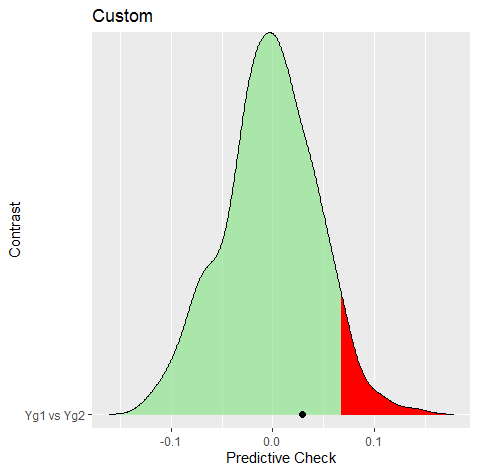
Predictive Check

The next step is to compute the observed difference and then perform the check.

# observed
obs <- f(Y_males, Y_females)

# check
ppc <- ggm_compare_ppc(Y_males, Y_females, 
                       iter = 250, 
                       FUN = f, 
                       custom_obs = obs)

# print
ppc

#> BGGM: Bayesian Gaussian Graphical Models 
#> --- 
#> Test: Global Predictive Check 
#> Posterior Samples: 250 
#>   Group 1: 896 
#>   Group 2: 1813 
#> Nodes:  5 
#> Relations: 10 
#> --- 
#> Call: 
#> ggm_compare_ppc(Y_males, Y_females, iter = 250, FUN = f, custom_obs = obs)
#> --- 
#> Custom: 
#>  
#>    contrast custom.obs p.value
#>  Yg1 vs Yg2      0.029   0.264
#> ---

Note this requires the user to determine $\alpha$ .

Plot

The check can also be plotted

plot(ppc)

where the red is the critical region.

Approach 3: Bayesian Hypothesis Testing

The above approaches cannot provide evidence that the sum is equal. In other words, just because there was not a difference, this does not provide evidence for equality. The Bayes factor methods allow for formally assessing the equality model, that is,

$\begin{align} \mathcal{H}_1&: (\rho^{male}_{A1--A2}\; + \; \rho^{male}_{A1--A3}) > (\rho^{female}_{A1--A2}\; + \; \rho^{female}_{A1--A3}) \\ \mathcal{H}_2&: (\rho^{male}_{A1--A2}\; + \; \rho^{male}_{A1--A3}) = (\rho^{female}_{A1--A2}\; + \; \rho^{female}_{A1--A3}) \\ \mathcal{H}_3&: \text{not} \; \mathcal{H}_1 \; \text{or} \; \mathcal{H}_2 \end{align}$

where $\mathcal{H}_3$ is the complement and can be understood as neither the first or second hypothesis.

Test Hypothesis

The hypothesis is easily translated to R code

hyp <- c("g1_A1--A2 + g1_A1--A3 > g2_A1--A2 + g2_A1--A3; 
          g1_A1--A2 + g1_A1--A3 = g2_A1--A2 + g2_A1--A3")

Note the g1 indicates the group and ; separates the hypotheses. I again assume the data is Gaussian (although this can be changed to type = "ordinal" or type = "mixed"; see here)

test <- ggm_compare_confirm(Y_males, Y_females, 
                            hypothesis = hyp)


# print
test


#> BGGM: Bayesian Gaussian Graphical Models 
#> Type: continuous 
#> --- 
#> Posterior Samples: 25000 
#>   Group 1: 896 
#>   Group 2: 1813 
#> Variables (p): 5 
#> Relations: 10 
#> Delta: 15 
#> --- 
#> Call:
#> ggm_compare_confirm(Y_males, Y_females, hypothesis = hyp)
#> --- 
#> Hypotheses: 
#> 
#> H1: g1_A1--A2+g1_A1--A3>g2_A1--A2+g2_A1--A3
#> H2: g1_A1--A2+g1_A1--A3=g2_A1--A2+g2_A1--A3
#> H3: complement
#> --- 
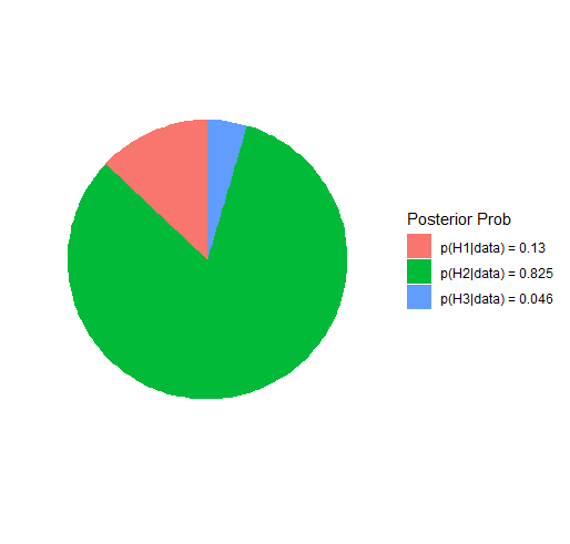
#> Posterior prob: 
#> 
#> p(H1|data) = 0.13
#> p(H2|data) = 0.825
#> p(H3|data) = 0.046
#> --- 
#> Bayes factor matrix: 
#>       H1    H2     H3
#> H1 1.000 0.158  2.853
#> H2 6.349 1.000 18.113
#> H3 0.351 0.055  1.000
#> --- 
#> note: equal hypothesis prior probabilities

Note the posterior hypothesis probability for the equality model is 0.825. The Bayes factor matrix then divides those values, for example, $BF_{21}$ indicates the data were about 6 times more likely under $\mathcal{H}_2$ than $\mathcal{H}_1$ .

Plot Hypothesis

The hypothesis can be plotted

plot(test)

Sensitivity Analysis

It is also important to check the robustness. Here the width of the prior distribution is decreased

test <- ggm_compare_confirm(Y_males, Y_females, 
                            hypothesis = hyp, 
                            prior_sd = 0.15)
# print
test$out_hyp_prob

#> 0.18523406 0.74906147 0.06570447

which results in a probability of 0.75 for $\mathcal{H}_2$ ( $BF_{21} = 4.04$ ).

Conclusion

Three approaches for testing the same hypothesis were demonstrated in this vignette. This highlights that any hypothesis can be tested in BGGM and in several ways.

References

Rodriguez, Josue E, Donald R Williams, Philippe Rast, and Joris Mulder. 2020. “On Formalizing Theoretical Expectations: Bayesian Testing of Central Structures in Psychological Networks.” PsyArXiv. https://doi.org/10.31234/osf.io/zw7pf.

Donny Williams

5/23/2020