Predictability: Binary, Ordinal, and Continuous

Background

This vignette describes a new feature to BGGM (2.0.0) that allows for computing network predictability for binary and ordinal data. Currently the available option is Bayesian $R^2$ (Gelman et al. 2019).

R packages

# need the developmental version
if (!requireNamespace("remotes")) { 
  install.packages("remotes")   
}   

# install from github
remotes::install_github("donaldRwilliams/BGGM")
library(BGGM)

Binary

The first example looks at Binary data, consisting of 1190 observations and 6 variables. The data are called women_math and the variable descriptions are provided in BGGM.

The model is estimated with

# binary data
Y <- women_math

# fit model
fit <- estimate(Y, type = "binary")

and then predictability is computed

r2 <- predictability(fit)

# print
r2

#> BGGM: Bayesian Gaussian Graphical Models 
#> --- 
#> Metric: Bayes R2
#> Type: binary 
#> --- 
#> Estimates:
#> 
#>  Node Post.mean Post.sd Cred.lb Cred.ub
#>     1     0.016   0.012   0.002   0.046
#>     2     0.103   0.023   0.064   0.150
#>     3     0.155   0.030   0.092   0.210
#>     4     0.160   0.021   0.118   0.201
#>     5     0.162   0.022   0.118   0.202
#>     6     0.157   0.028   0.097   0.208
#> ---

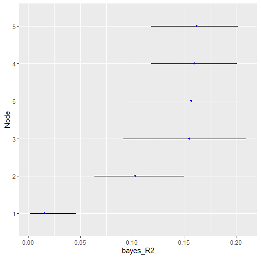
There are then two options for plotting. The first is with error bars, denoting the credible interval (i.e., cred),

plot(r2,
     type = "error_bar",
     size = 4,
     cred = 0.90)

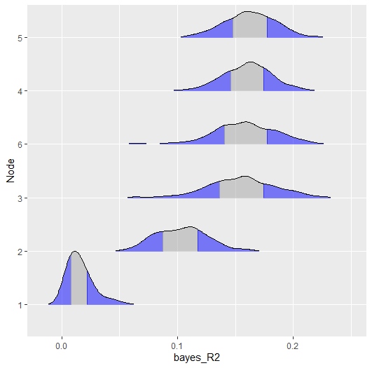
and the second is with a ridgeline plot

plot(r2,
     type = "ridgeline",
     cred = 0.50)

Ordinal

In the following, the ptsd data is used (5-level Likert). The variable descriptions are provided in BGGM. This is based on the polychoric partial correlations, with $R^2$ computed from the corresponding correlations (due to the correspondence between the correlation matrix and multiple regression).

Y <- ptsd

fit <- estimate(Y + 1, type = "ordinal")

The only change is switching type from "binary to ordinal. One important point is the + 1. This is required because for the ordinal approach the first category must be 1 (in ptsd the first category is coded as 0).

r2 <- predictability(fit)

# print 
r2 

#> BGGM: Bayesian Gaussian Graphical Models 
#> --- 
#> Metric: Bayes R2
#> Type: ordinal 
#> --- 
#> Estimates:
#> 
#>  Node Post.mean Post.sd Cred.lb Cred.ub
#>     1     0.487   0.049   0.394   0.585
#>     2     0.497   0.047   0.412   0.592
#>     3     0.509   0.047   0.423   0.605
#>     4     0.524   0.049   0.441   0.633
#>     5     0.495   0.047   0.409   0.583
#>     6     0.297   0.043   0.217   0.379
#>     7     0.395   0.045   0.314   0.491
#>     8     0.250   0.042   0.173   0.336
#>     9     0.440   0.048   0.358   0.545
#>    10     0.417   0.044   0.337   0.508
#>    11     0.549   0.048   0.463   0.648
#>    12     0.508   0.048   0.423   0.607
#>    13     0.504   0.047   0.421   0.600
#>    14     0.485   0.043   0.411   0.568
#>    15     0.442   0.045   0.355   0.528
#>    16     0.332   0.039   0.257   0.414
#>    17     0.331   0.045   0.259   0.436
#>    18     0.423   0.044   0.345   0.510
#>    19     0.438   0.044   0.354   0.525
#>    20     0.362   0.043   0.285   0.454
#> ---

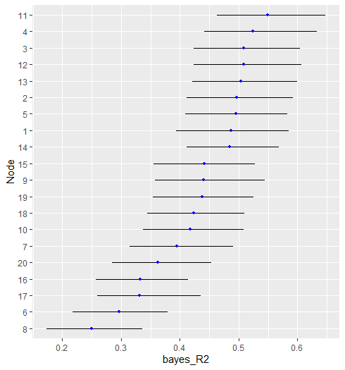
Here is the error_bar plot.

plot(r2)

Note that the plot object is a ggplot which allows for further customization (e.g,. adding the variable names, a title, etc.).

Continuous

It is quite common to compute predictability assuming that the data are Gaussian. In the context of Bayesian GGMs, this was introduced in (Williams 2018). This can also be implemented in BGGM.

# fit model
fit <- estimate(Y)

# predictability
r2 <- predictability(fit)

type is missing which indicates that continuous is the default.

Note

$R^2$ for binary and ordinal data is computed for the underlying latent variables. This is also the case when type = "mixed (a semi-parametric copula). In future releases, there will be support for predicting the variables on the observed scale.

References

Gelman, Andrew, Ben Goodrich, Jonah Gabry, and Aki Vehtari. 2019. “R-squared for Bayesian Regression Models.” American Statistician 73 (3): 307–9.

Williams, Donald R. 2018. “Bayesian Estimation for Gaussian Graphical Models: Structure Learning, Predictability, and Network Comparisons.” arXiv. https://doi.org/10.31234/OSF.IO/X8DPR.

Donny Williams