GGM: Exploratory Hypothesis Testing

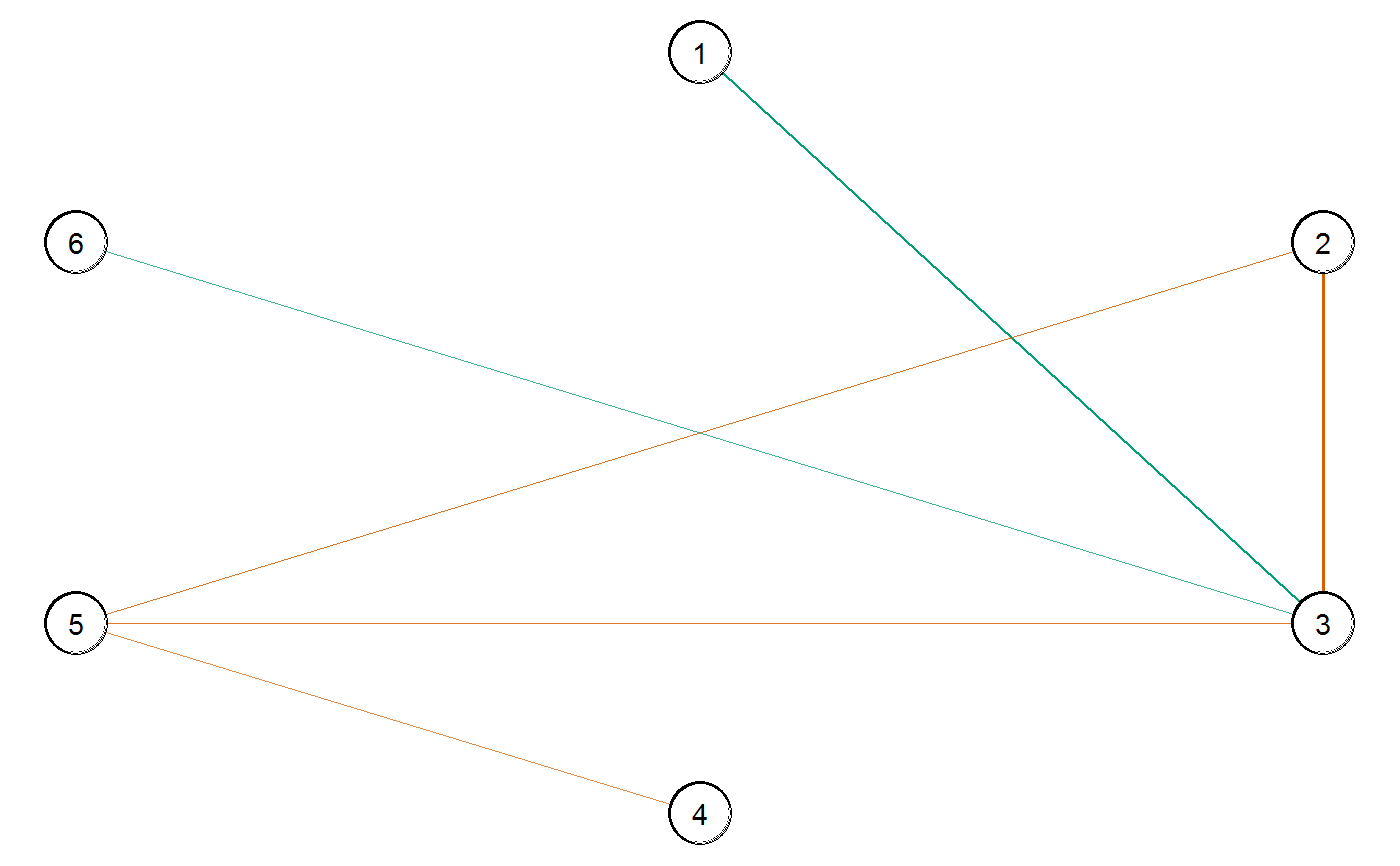
Learn the conditional (in)dependence structure with the Bayes factor using the matrix-F prior distribution (Mulder and Pericchi 2018) . These methods were introduced in Williams and Mulder (2019) . The graph is selected with select.explore and then plotted with plot.select.

explore(
  Y,
  formula = NULL,
  type = "continuous",
  mixed_type = NULL,
  analytic = FALSE,
  prior_sd = 0.25,
  iter = 5000,
  progress = TRUE,
  impute = TRUE,
  seed = 1,
  ...
)

Arguments

Y	Matrix (or data frame) of dimensions n (observations) by p (variables).
formula	An object of class `formula`. This allows for including control variables in the model (i.e., `~ gender`).
type	Character string. Which type of data for `Y` ? The options include `continuous`, `binary`, `ordinal`, or `mixed` (semi-parametric copula). See the note for further details.
mixed_type	Numeric vector. An indicator of length p for which varibles should be treated as ranks. (1 for rank and 0 to assume normality). The default is to treat all integer variables as ranks when `type = "mixed"` and `NULL` otherwise. See note for further details.
analytic	Logical. Should the analytic solution be computed (default is `FALSE`)? (currently not implemented)
prior_sd	Scale of the prior distribution, approximately the standard deviation of a beta distribution (defaults to 0.25).
iter	Number of iterations (posterior samples; defaults to 5000).
progress	Logical. Should a progress bar be included (defaults to `TRUE`) ?
impute	Logicial. Should the missing values (`NA`) be imputed during model fitting (defaults to `TRUE`) ?
seed	An integer for the random seed.
...	Currently ignored (leave empty).

Value

The returned object of class explore contains a lot of information that is used for printing and plotting the results. For users of BGGM, the following are the useful objects:

pcor_mat partial correltion matrix (posterior mean).
post_samp an object containing the posterior samples.

Details

Controlling for Variables:

When controlling for variables, it is assumed that Y includes only the nodes in the GGM and the control variables. Internally, only the predictors that are included in formula are removed from Y. This is not behavior of, say, lm, but was adopted to ensure users do not have to write out each variable that should be included in the GGM. An example is provided below.

Mixed Type:

The term "mixed" is somewhat of a misnomer, because the method can be used for data including only continuous or only discrete variables. This is based on the ranked likelihood which requires sampling the ranks for each variable (i.e., the data is not merely transformed to ranks). This is computationally expensive when there are many levels. For example, with continuous data, there are as many ranks as data points!

The option mixed_type allows the user to determine which variable should be treated as ranks and the "emprical" distribution is used otherwise. This is accomplished by specifying an indicator vector of length p. A one indicates to use the ranks, whereas a zero indicates to "ignore" that variable. By default all integer variables are handled as ranks.

Dealing with Errors:

An error is most likely to arise when type = "ordinal". The are two common errors (although still rare):

The first is due to sampling the thresholds, especially when the data is heavily skewed. This can result in an ill-defined matrix. If this occurs, we recommend to first try decreasing prior_sd (i.e., a more informative prior). If that does not work, then change the data type to type = mixed which then estimates a copula GGM (this method can be used for data containing only ordinal variable). This should work without a problem.
The second is due to how the ordinal data are categorized. For example, if the error states that the index is out of bounds, this indicates that the first category is a zero. This is not allowed, as the first category must be one. This is addressed by adding one (e.g., Y + 1) to the data matrix.

Imputing Missing Values:

Missing values are imputed with the approach described in Hoff (2009) . The basic idea is to impute the missing values with the respective posterior pedictive distribution, given the observed data, as the model is being estimated. Note that the default is TRUE, but this ignored when there are no missing values. If set to FALSE, and there are missing values, list-wise deletion is performed with na.omit.

Note

Posterior Uncertainty:

A key feature of BGGM is that there is a posterior distribution for each partial correlation. This readily allows for visiualizing uncertainty in the estimates. This feature works with all data types and is accomplished by plotting the summary of the explore object (i.e., plot(summary(fit))). Note that in contrast to estimate (credible intervals), the posterior standard deviation is plotted for explore objects.

"Default" Prior:

In Bayesian statistics, a default Bayes factor needs to have several properties. I refer interested users to section 2.2 in Dablander et al. (2020) . In Williams and Mulder (2019) , some of these propteries were investigated including model selection consistency. That said, we would not consider this a "default" (or "automatic") Bayes factor and thus we encourage users to perform sensitivity analyses by varying the scale of the prior distribution.

Furthermore, it is important to note there is no "correct" prior and, also, there is no need to entertain the possibility of a "true" model. Rather, the Bayes factor can be interpreted as which hypothesis best (relative to each other) predicts the observed data (Section 3.2 in Kass and Raftery 1995) .

Interpretation of Conditional (In)dependence Models for Latent Data:

See BGGM-package for details about interpreting GGMs based on latent data (i.e, all data types besides "continuous")

References

Dablander F, Bergh Dvd, Ly A, Wagenmakers E (2020). “Default Bayes Factors for Testing the (In) equality of Several Population Variances.” arXiv preprint arXiv:2003.06278.

Hoff PD (2009). A first course in Bayesian statistical methods, volume 580. Springer.

Kass RE, Raftery AE (1995). “Bayes Factors.” Journal of the American Statistical Association, 90(430), 773--795.

Mulder J, Pericchi L (2018). “The Matrix-F Prior for Estimating and Testing Covariance Matrices.” Bayesian Analysis, 1--22. ISSN 19316690, doi: 10.1214/17-BA1092 .

Williams DR, Mulder J (2019). “Bayesian Hypothesis Testing for Gaussian Graphical Models: Conditional Independence and Order Constraints.” PsyArXiv. doi: 10.31234/osf.io/ypxd8 .

Examples

# \donttest{
# note: iter = 250 for demonstrative purposes

###########################
### example 1:  binary ####
###########################
Y <- women_math[1:500,]

# fit model
fit <- explore(Y, type = "binary",
                iter = 250,
                progress = FALSE)

# summarize the partial correlations
summ <- summary(fit)

# plot the summary
plt_summ <- plot(summary(fit))

# select the graph
E <- select(fit)

# plot the selected graph
plt_E <- plot(E)

plt_E$plt_alt
# }