Introduction
This is a follow-up to the vignette “Three
Ways to Test the Same Hypothesis”. A new feature,
pcor_sum, was added to BGGM that allows
for testing partial correlation sums. This differs from the Bayes factor
approach (“Approach #3”), in that only the posterior distribution is
used to determine whether there is a difference in the sums.
R package
# need the developmental version
if (!requireNamespace("remotes")) {
  install.packages("remotes")
}

# install from github
remotes::install_github("donaldRwilliams/BGGM")
library(BGGM)
One Group
This first example looks at one group, where a sum is tested within
the same ptsd network. I focus on the relations between the
re-experiencing (B) and avoidance (C)
communities. In particular, the sum of relations between the “Intrusion”
(5 nodes) community and the “Avoidance” (two nodes) community is
tested.
Sum to String
For the avoidance symptom “avoidance of thoughts” C1,
this can be written in R code with
# ptsd
Y <- ptsd

# paste together sums
paste0(colnames(Y)[1:5],  "--C1", collapse = " + ")

#> "B1--C1 + B2--C1 + B3--C1 + B4--C1 + B5--C1"
whereas, for the avoidance symptom “avoidance of reminders”
(C2), this is written as
paste0(colnames(Y)[1:5],  "--C2", collapse = " + ")

#> "B1--C2 + B2--C2 + B3--C2 + B4--C2 + B5--C2"
Note that typically this would have to be written out.
paste0 was used in this case to avoid typing out all of the
relations.
Fit Model
Here an ordinal GGM is fitted
fit <- estimate(Y+1, type = "ordinal", iter = 1000)where the +1 changes the first category from 0 to 1
(required).
Test Sums
The next step is to use the pcor_sum function. First, I
combine the sums into one string separated with ;.
# sum 1
sum1 <- paste0(colnames(Y)[1:5],  "--C1", collapse = " + ")

# sum 2
sum2 <- paste0(colnames(Y)[1:5],  "--C2", collapse = " + ")

# paste together
sums <- paste(sum1, sum2, sep = ";")

# print
sums
#> "B1--C1 + B2--C1 + B3--C1 + B4--C1 + B5--C1;B1--C2 + B2--C2 + B3--C2 + B4--C2 + B5--C2"
Next pcor_sum is used
test_sum <- pcor_sum(fit, relations = sums)

# print
test_sum

# BGGM: Bayesian Gaussian Graphical Models
# ---
# Network Stats: Posterior Sum
# Posterior Samples: 1000
# ---
# Estimates
#
# Sum:
#                                    Post.mean Post.sd Cred.lb Cred.ub
# B1--C1+B2--C1+B3--C1+B4--C1+B5--C1     0.215   0.096   0.034   0.404
# B1--C2+B2--C2+B3--C2+B4--C2+B5--C2     0.334   0.097   0.145   0.514
# ---
#
# Difference:
# B1--C1+B2--C1+B3--C1+B4--C1+B5--C1 - B1--C2+B2--C2+B3--C2+B4--C2+B5--C2
#
#  Post.mean Post.sd Cred.lb Cred.ub Prob.greater Prob.less
#     -0.119   0.145  -0.409   0.173        0.205     0.795
# ---
Prob.greater is the posterior probability that the first
sum is larger than the second sum.
Plot Results
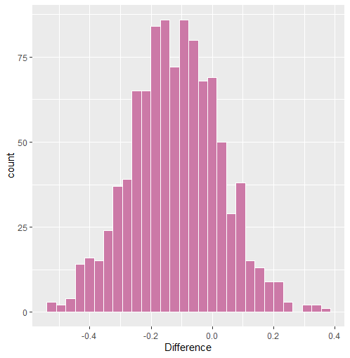
The object test_sum can then be plotted. Note this
returns three plots, but only the difference is shown here
plot(test_sum)$diff
The histogram is not very smooth in this case because
iter = 1000, but this of course can be changed.
Two Groups
This next example is for two groups. The data are called
bfi and they are in the BGGM package. I
compare a sum of two relations for questions measuring agreeableness in
males and females. The relations tested are as follows
Sum to String
sums <- c("A3--A4 + A4--A5")where A1 is “know how to comfort others”,
A4 is “love children”, and A5 is “make people
feel at ease”.
Test Sums
Then test the sum
test_sum <- pcor_sum(fit_female, fit_male, relations = sums)

# print
test_sum

#> BGGM: Bayesian Gaussian Graphical Models
#> ---
#> Network Stats: Posterior Sum
#> Posterior Samples: 5000
#> ---
#> Estimates
#>
#> Sum:
#>                   Post.mean Post.sd Cred.lb Cred.ub
#> g1: A3--A4+A4--A5     0.292   0.026   0.241   0.342
#> g2: A3--A4+A4--A5     0.305   0.036   0.234   0.375
#> ---
#>
#> Difference:
#> g1: A3--A4+A4--A5 - g2: A3--A4+A4--A5
#>
#>  Post.mean Post.sd Cred.lb Cred.ub Prob.greater Prob.less
#>     -0.014   0.045    -0.1   0.074        0.386     0.614
#> --- Notes
By default, the print function for pcor_sum provides 95
% credible intervals. This can be changed by directly using the print
function, for example print(test_sum, cred = 0.99),
provides 99 % credible intervals.
Currently, this function only supports sums, due to this being of interest for the psychological network literature in particular. This can be extended to accommodate multiplication, subtraction, testing values other than zero, etc. Please make a feature request at either github or BGGM-users group.
