GGM: Missing Data — bggm

Estimation and exploratory hypothesis testing with missing data.

Usage

bggm_missing(x, iter = 2000, method = "estimate", ...)

Arguments

x: An object of class mid mice.
iter: Number of iterations for each imputed dataset (posterior samples; defaults to 2000).
method: Character string. Which method should be used (default set to estimate)? The current options are "estimate" and "explore".
...: Additional arguments passed to either estimate or explore.

Value

An object of class estimate or explore.

Note

Currently, BGGM is compatible with the package mice for handling the missing data. This is accomplished by fitting a model for each imputed dataset (i.e., more than one to account for uncertainty in the imputation step) and then pooling the estimates.

In a future version, an additional option will be added that allows for imputing the missing values during model fitting. This option will be incorporated directly into the estimate or explore functions, such that bggm_missing will always support missing data with mice.

Support:

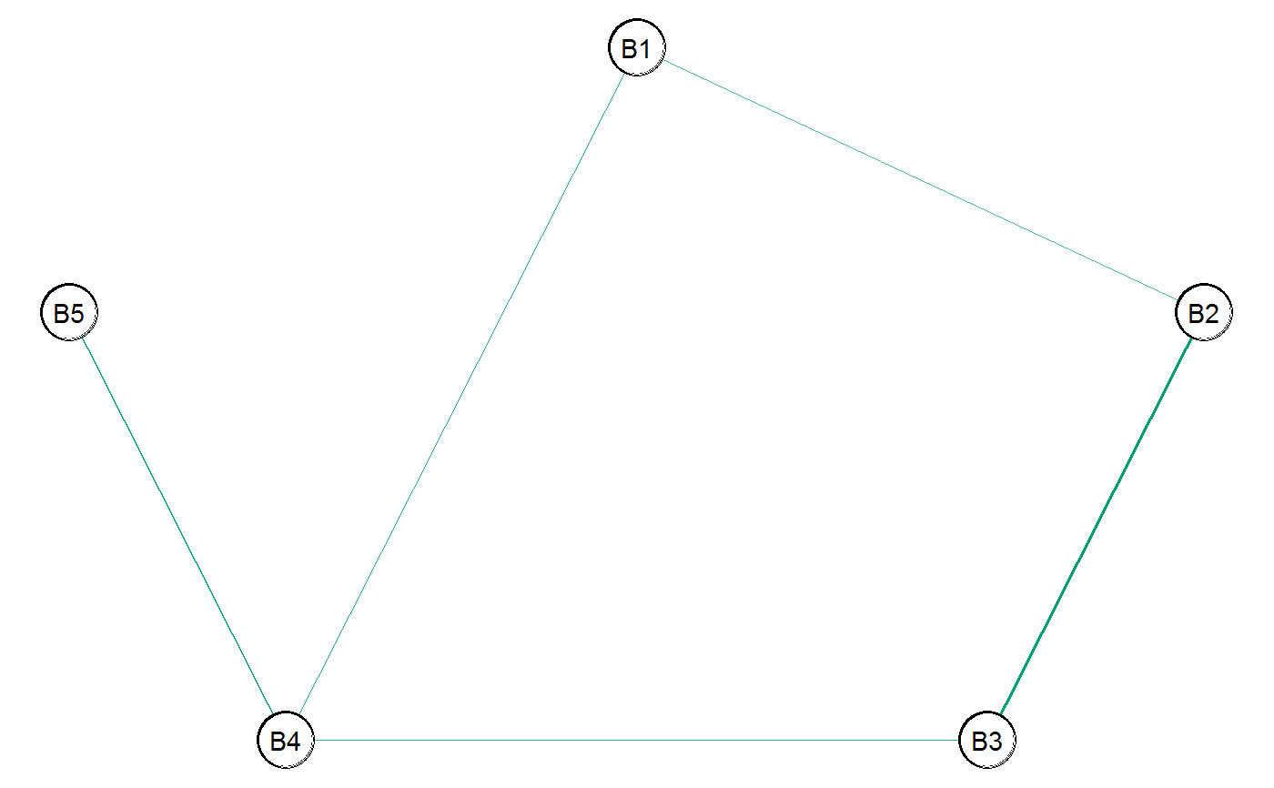
There is limited support for missing data. As of version 2.0.0, it is possible to determine the graphical structure with either estimate or explore, in addition to plotting the graph with plot.select. All data types are currently supported.

Memory Warning: A model is fitted for each imputed dataset. This results in a potentially large object.

Examples

# \donttest{
# note: iter = 250 for demonstrative purposes

# need this package
library(mice, warn.conflicts = FALSE)

# data
Y <- ptsd[,1:5]

# matrix for indices
mat <- matrix(0, nrow = 221, ncol = 5)

# indices
indices <- which(mat == 0, arr.ind = TRUE)

# Introduce 50 NAs
Y[indices[sample(1:nrow(indices), 50),]] <- NA

# impute
x <- mice(Y, m = 5, print = FALSE)

#########################
#######   copula    #####
#########################
# rank based parital correlations

# estimate the model (following code commented due to CRAN checks) 
fit_est <-  bggm_missing(x,
                         method = "estimate",
                         type =  "mixed",
                         iter = 250,
                         progress = FALSE)

# select edge set
E <- select(fit_est)

# plot E
plt_E <- plot(E)$plt

plt_E

# }